What are Steerable Neural Networks and context
Introduction
Geometrical deep learning, as a branch of Deep Learning, aims to extend traditional AI frameworks such as Convolutional Neural Networks to process 3D or 2D geometric objects represented as graphs, manifolds, or point clouds. By incorporating geometric relationships and spatial dependencies directly into the learning framework, geometrical deep learning harnesses the inherent structural properties of data to eliminate the requirement for memory-intensive data augmentation techniques. For all these reasons, Geometrical Deep Learning can be seen as valuable tool for tackling complex data scenarios in domains such as computer vision, natural language processing, and beyond. Concerning the type of task and the type of transformation, a large variety of new CNN architectures have been proposed so far as “Spherical Neural Networks” (link), “Graph Neural Networks” (link), and “Steerable Neural Networks”.
This tutorial will present an introduction to “Steerable Neural Networks” (S-CNNs), trying to convey an intuitive understanding of the mathematical concepts behind them and a step-by-step explanation on how to design these networks.
The tutorial is composed of two articles. This first article serves as an introduction to steerable neural networks (NNs), explaining their purpose and delving deeper into the concepts and formalism underlying S-CNNs. The second article (here) discusses at a high level the design of steerable filters and the steerable networks as overall.
This work aims at filling the gap between the current scientific literature and the wider data science audience. It is ideal for tech professionals as well as for researchers in this new branch of machine learning.
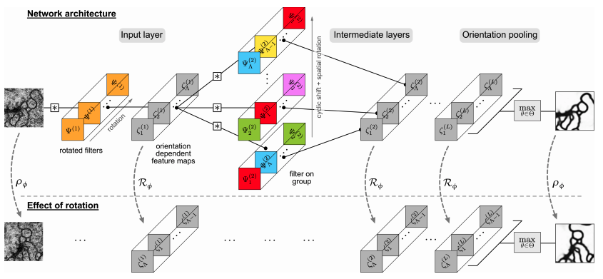
Example of a simple Steerable Neural Network taken from the paper [3]. As possible to see the effect of rotation in the input image is reflected to the the output response of the network.
The following papers are taken as reference:
[1] “3D Steerable CNNs: Learning Rotationally Equivariant Features in Volumetric Data”, Weilier et al., (link);
[2] “Steerable CNNs”, Cohen et al. ( link);
[3] “Learning Steerable Filters for Rotation Equivariant CNNs”,Weilier et al., (link)
[4] “General E(2)-Equivariant Steerable CNNs” Weilier et al., (link)
[5] “Scale Steerable Filters for the Locally Scale-Invariant Convolutional Neural Network”, Ghosh et al. (link)
[6] “A program to build E -equivariant steerable CNNs.” Cesa et al. (link)
What are Steerable Neural Networks:
Steerable neural networks take their name from the particular type of filters they use. Such filters are called g-steerable filters and they have been inspired by the steerable filters which gained popularity in the image recognition field for edge detection or oriented texture analysis at the beginning of the 90’s. Steerable means commonly dirigible, manageable, capable of being managed or controlled. Following this convention, the response of a steerable filters is orientable and adaptable to a specific orientation of the input (an image for example). Steerability is related to another very important property which is called Equivariance. In an equivariant filter, if the INPUT to the filter is transformed according to a precise and well-defined geometric transformation g (translation, rotation, shift), the OUTPUT (which results from the convolution of the INPUT with the filter) is transformed by the same transformation g. In general, equivariance does not require that the transformations (the one at the input and the one at the output) are the same. This concept will be better addressed in the next paragraph but for now it allows us to provide a first definition of steerable filter and steerable CNN.
A Steerable CNN filter can be defined as a filter whose kernel is structured as a concatenation of different steerable filters. These filters show equivariance properties in relation to the operation of convolution with respect to a set of well-defined geometric transformations.
As we can see later, the condition of equivariance on the convolution operation leads to the imposition of specific constraints over the structure of the kernel and on its weights. From this definition it is now possible to define what a steerable CNN is: Steerable Neural Networks are neural networks composed of a series of steerable filters.
What are S-CNN used for:
The strength of a normal CNN is in its equivariance to translation. However, Steerable NN’s are more flexible and can show other types of transformations, rotation. In a rotationally equivariant problem, an unmodified CNN is compelled to learn rotated versions of the same filter introducing a redundant degree of freedom and increasing the risk of overfitting.
For this reason, Steerable CNN networks can outperform the classical CNN by directly incorporating information about the geometrical transformations acting at the input. This property makes S-CNNs particularly useful for several challenging tasks where we have to process inputs that have a geometrical description and representation such as images, manifolds, or vector fields.
Possible practical applications are for example :

Example of application of a a 3D steerable neural network for 3D object recognition. The input object (on the top) , and the representation of two different hidden layers feature maps. Taken from Link
Preliminary definitions and Context
After introducing Steerable Neural Networks and their applications, let’s dive into the theory behind them. This section offers a more formal explanation of equivariance and steerability, providing essential definitions and a formal framework that will be instrumental in understanding the construction of steerable filters in the subsequent article.
This article relies on an understanding of maps and geometrical transformations, for more information look on this other article.
1. EQUIVARIANCE:
Equivariance is a property of particular interest in symmetric problems. As stated before, in an equivariant model when the input is acted on by the transformation, it also acts on the output such that the application of the transformation can be applied before or after the model’s application with no change in overall behaviour. In an everyday setting there are many examples of equivariance. For example, when driving, the direction in which a car steers when the wheel is turned is equivariant with respect to the direction the car is pointing. Formally, if we have a map ?: X → Y, where X⊂ℝᵈ and Y⊂ℝᵈ¹ , and g, a geometrical transformation belonging to the group G, ? is equivariant to G if :

Eq.1: Math equation representing the equivariance of ? with respect to g.
where Π₀(g) : X → X’ and Π₁(g): Y→ Y’ are two linear maps ( e.g. often matrices applied by multiplication) determined by the application of g to x. A visual example is given by the picture below taken from the paper [2]. In the image g is a rotation, specifically “rotation of -90°”; it is, therefore, denominated r. Π₀(r) operates in the domain of ? (=X), while Π₁(r) works in the codomain of ? (=Y).
If X=ℝ², 2-D cartesian space, and r is the transformation “clock-wise rotation of 90°”, the matrix Π₀(r) would be equal to a 2x2 Euler matrix with θ=π/2.
One should notice that if ? is equivariant with respect to G, applying a transformation and then computing the map produces the same result as calculating the map and then applying the transformation, a property formerly known as commutation.
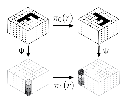
Fig2A: A visual example of a function Ѱ equivariant to a transformation r. Taken from article [2].
At this point it is also worth mentioning a special case. Invariance, a particular type of equivariance where X=X’ and Y=Y’. In whatever way the input is transformed, the output always remains the same. From a deep learning prospective, invariant filter could be useful for example for object recognition: however an input image is rotated the output of the filter remains the same. One should note that the spaces X and Y may not necessarily have the same dimensionality, for example if we are trying to determine the orientation (Y as a 2-vector) of a car in a picture (X as a 2-d array of pixels), then the transformations Π₁(g) and Π₀(g) will be different as they apply to different spaces, even when they share the same g.
2. STEERABLE FILTERs:
In contrast to the steerability of a car, steerable filters are a little more challenging to intuit. Both, however, share the underlying goal of achieving a consistent and predictable response to a specific parameter — a response that is intimately linked to the inherent transformations of the filter itself.
An intuitive example might be the following: think of a wind vane on a rooftop that shows the direction of the wind. Instead of installing a separate sensor for every possible wind direction, which would be impractical, you have a wind vane that rotates to align with the current wind direction.A steerable filter is like a wind vane. It adapts to directions encoded in input signals without needing a unique sensor for each possibility. In the same way, steerable filters in image processing adapt to different features or orientations in an image without requiring a separate filter for every possible orientation of the input. This approach offers an intelligent and effective method for modeling systems. In the context of machine learning, it enables us to concentrate on constructing valuable models without worrying about augmentation or incorporating additional weights to handle different orientations.
While steerability can be applied generally to any set of transformations, we will here use rotations to introduce the idea in a more formal way.
Let ?: ℝᵈ →ℝᵈ¹ be a convolution map whose kernel function is k.
Be x∈ℝⁿ , given an input signal depending on x , f(x) ∈ ℝᵈ, and output signal , f ₁(x) ∈ ℝᵈ¹ , we can write: f ₁(x)= ?( f(x)) which means f ₁(x)= k(x) ∗ f(x) .
This filter is defined steerable with respect to rotations if :
(1) its convolution kernel k(x) of each output element, can be expressed as a sum of basis functions ψⱼ(x), j=1,..M.
(2) the filter’s rotation by an arbitrary angle θ , g_θ, can be expressed in terms of rotations applied to each single basis function (this is valid for each θ). In mathematical terms it means:

Eq.2: Definition of Steerable filter
Thanks to this property, it is possible to uniquely orient the filter’s response to an input, by modifying the values of wⱼ. Let’s provide an example.
The simplest illustration of a single steerable filter is in 2D space a filter whose kernel function is the directional derivative of a two-dimensional Gaussian. In this case the k: ℝ² →ℝ and x = (x₁,x₂) ∈ ℝ² :


Eq.3: Directional derivative of a two-dimensional Gaussian (above) and transformation of a function k R² →R under gθ.
In the following lines we will show that this filter is steerable in the sense explained above.
From the theory we know that, given that k codomain is ℝ, we can write the rotated filter as Eq.3 (for more info look at Eq.3 in the next session).
By developing this equation we can show the steerability:
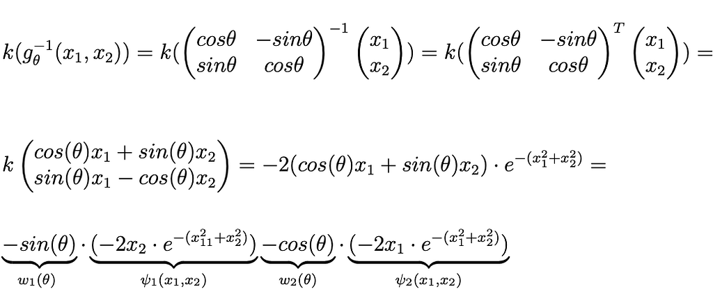
Eq.5: Mathematical proof of steerability of a the directional derivative of a two-dimensional Gaussian
In this case we have applied the transformation g_θ: ℝ²→ℝ² and it is represented by the 2D euler matrix (see later induced representation). If we calculate k(g_θ ⁻¹(x₁,x₂)), we can see, after some algebra, that the generic rotated version of this impulsive filter can be expressed as a linear combination of two basis functions ѱ₁(x₁,x₂) and ѱ₂(x₁,x₂) with coefficient parameterized by θ.
As possible to see in the equation reported below (Eq.6) , given the linearity of convolution, it is always possible to express the convolution of an input function f with the θ-rotated impulsive response g_θ(k(x,y))=k_θ as a linear combination of the convolutions of f with the single basis ѱ₁,ѱ₂ of k.

Eq.6: Convolution of a steerable filter with f.
This formula highlights the power of steerable filters in a neural network.
By incorporating these filters, we have the potential to construct a steerable kernel that ‘steers’ its responses to the orientation of the input. Each basis function acts like a versatile tool, permitting the network to efficiently blend these functions using learned weights ‘w₁’ and ‘w₂’ to respond accurately to varying orientations. For instance, when the network encounters data with varying orientations, such as a rotated object in an image, it configures these weights to align the kernel’s responses to the orientation of the input data. This adaptability enhances efficiency and effectiveness, leading to the same or better outcomes with fewer parameters. For this reason this approach can be used as the foundation for a more powerful CNN using steerable properties to handle diverse input orientations.
Specifically, in next article, we’ll explore this further and see how a we can use the concept of steerable filter to build equivariant filters.
However, before we dive in, some definitions in this context will provide clarity and aid our discussion. For this reason in the next paragraph we introduce some formalism around convolution.
3. FORMALISM:
In this part, we try to give to the reader a schematic explanation of all the elements considered in the analysis. This formalism will allow us to define more formally a CNN and the geometrical transformations which operate at the input level. This will allow us in the next article to understand how Steerable CNNs work.
The elements:
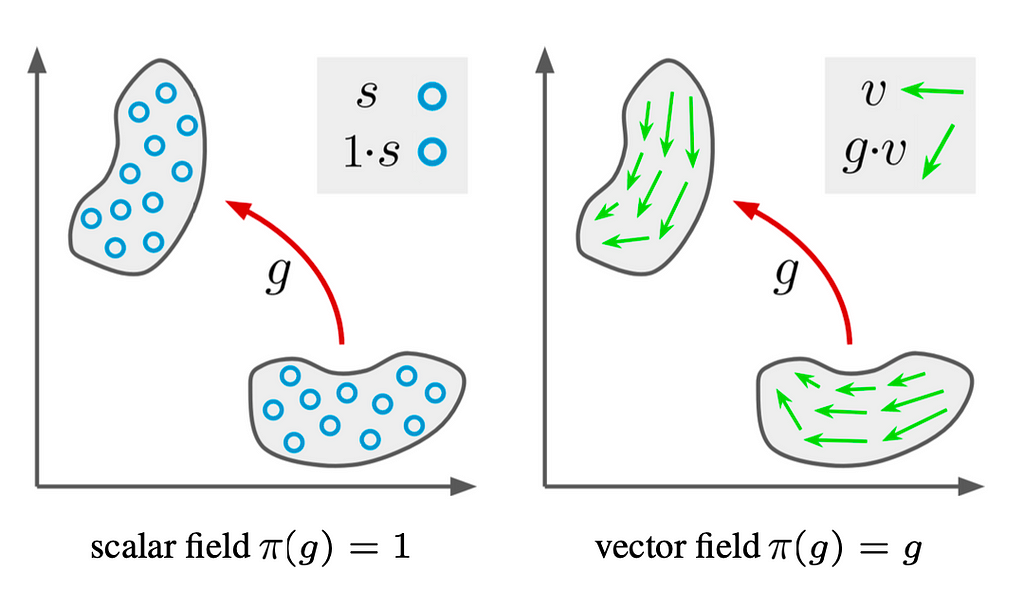
Fig 2B: graphical representation of the application of a transformation g on a scalar field (left) or on a vector field (right). Taken from paper [3].

Eq.7: how f is transformed by the application of the transformation g to x
In this case, the kernel can be seen as a function k: S → ℝ ͨ ʿⁿ ʾ ˟ ͨ ʿⁿ⁺ ¹ ʾ, where each position in S is connected to a matrix of dimension cʿⁿ ʾ ˟ cʿⁿ⁺ ¹ ʾ. For clarity, cⁿ and cⁿ ⁺ ¹ are respectively the dimension (number of features) of Fₙ and Fₙ₊₁.
We can define the convolution as following:


Eq.8: Top: Relation which connects layer n and layer n+1. Down: Definition of convolution in the space S
The top equation Eq.8 represents the function which connects the layer n and n+1; the one below is the definition of convolution in n-dimensional space S. The function σ(x) represents the non-linear function applied at the output of the convolution.
In Fig 2B, it is possible to see how, in a discrete domain, the convolution between the kernel and the input layer is calculated.Let’s illustrate this with a grayscale image denoted as f ₀: ℝ² -> ℝ. We can apply the filter discussed in Section 2, which was a steerable filter with the function
k(x₁, x₂) being a 2D Gaussian filter defined as k: ℝ² -> ℝ¹˟¹=ℝ.
In this case the application of the filter k on f₀ is the classical 2D convolution and it can be written as:

Eq.9: Definition of convolution
Differently, in Fig. 2B you can see another example where f ₀: ℝ²-> ℝ³ (rgb image for example) and f₁: ℝ²-> ℝ² and k₀: ℝ²-> ℝ³ ˟ ².
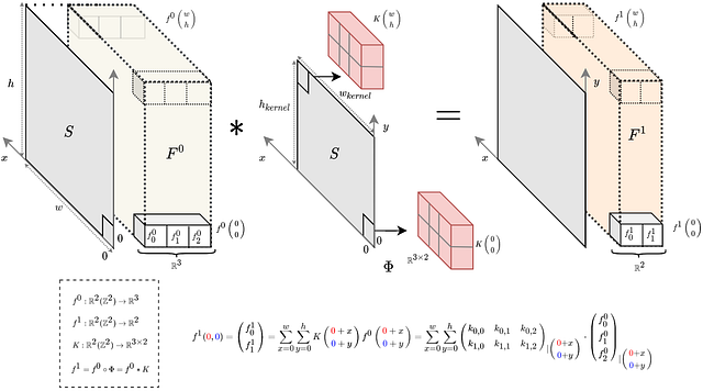
Fig 2B: Visual example of filter convolution as defined above having S=R². F⁰ is the input space where the signal f⁰ exists, in this case R³. As possible to notice, the convolution operation has been substitute by correlation operation as suggested in [4]
Combining all the points we’ve discussed so far, one can visualize a neural network within this formalism. Each individual feature map can be interpreted as a function f: S → Fₙ, where Fₙ= ℝʿⁿ ʾ and f₀(x) represents the network’s input. The filter’s application involves convolving it with its kernel function defined in Eq.8. It’s worth noting that the main innovation thus far lies in the geometric representation of f as a function operating in a positional space S, and the definition of convolution within this space.
Below, we provide a representation of what a neural network in this context looks like:

Eq.10: Symbolic representation of a neural network using the formalism expressed above.
We will understand in the next article how the definition of such formalism will help us in the design of a steerable CNN filter.
Conclusions
In this initial segment of our Steerable Neural Networks tutorial, we have established the fundamental concepts of Steerable Neural Networks, equivariance, and steerable filters. A mathematical framework has also been introduced to provide a rigorous foundation for understanding these concepts. Equivariance preserves behavior under transformations, while steerable filters adapt intelligently to input orientations. This groundwork paves the way for designing equivariant CNN filters, enhancing edge detection and orientation-based recognition. The next article will leverage these concepts for a deeper dive into Steerable CNN filters’ mechanics, completing our journey into this powerful neural network paradigm.
✍️ ?. About the authors:
1️⃣ Matteo Ciprian, Machine Learning Engineer/Researcher
2️⃣ Robert Schoonmaker, Signal Processing/Machine Learning Researcher

A gentle introduction to Steerable Neural Networks (part 1) was originally published in Towards Data Science on Medium, where people are continuing the conversation by highlighting and responding to this story.
Introduction
Geometrical deep learning, as a branch of Deep Learning, aims to extend traditional AI frameworks such as Convolutional Neural Networks to process 3D or 2D geometric objects represented as graphs, manifolds, or point clouds. By incorporating geometric relationships and spatial dependencies directly into the learning framework, geometrical deep learning harnesses the inherent structural properties of data to eliminate the requirement for memory-intensive data augmentation techniques. For all these reasons, Geometrical Deep Learning can be seen as valuable tool for tackling complex data scenarios in domains such as computer vision, natural language processing, and beyond. Concerning the type of task and the type of transformation, a large variety of new CNN architectures have been proposed so far as “Spherical Neural Networks” (link), “Graph Neural Networks” (link), and “Steerable Neural Networks”.
Steerable Neural Networks have garnered significant interest due to their unique ability to extend the capabilities of regular Convolutional Neural Networks (CNNs). These networks can be viewed as an evolution of CNNs, where the kernel is conditioned to satisfy specific constraints. While CNNs excel at being equivariant to translation, Steerable Neural Networks take it a step further by offering enhanced flexibility and capturing a wider range of transformations, such as rotation.
This tutorial will present an introduction to “Steerable Neural Networks” (S-CNNs), trying to convey an intuitive understanding of the mathematical concepts behind them and a step-by-step explanation on how to design these networks.
The tutorial is composed of two articles. This first article serves as an introduction to steerable neural networks (NNs), explaining their purpose and delving deeper into the concepts and formalism underlying S-CNNs. The second article (here) discusses at a high level the design of steerable filters and the steerable networks as overall.
This work aims at filling the gap between the current scientific literature and the wider data science audience. It is ideal for tech professionals as well as for researchers in this new branch of machine learning.

Example of a simple Steerable Neural Network taken from the paper [3]. As possible to see the effect of rotation in the input image is reflected to the the output response of the network.
The following papers are taken as reference:
[1] “3D Steerable CNNs: Learning Rotationally Equivariant Features in Volumetric Data”, Weilier et al., (link);
[2] “Steerable CNNs”, Cohen et al. ( link);
[3] “Learning Steerable Filters for Rotation Equivariant CNNs”,Weilier et al., (link)
[4] “General E(2)-Equivariant Steerable CNNs” Weilier et al., (link)
[5] “Scale Steerable Filters for the Locally Scale-Invariant Convolutional Neural Network”, Ghosh et al. (link)
[6] “A program to build E
What are Steerable Neural Networks:
Steerable neural networks take their name from the particular type of filters they use. Such filters are called g-steerable filters and they have been inspired by the steerable filters which gained popularity in the image recognition field for edge detection or oriented texture analysis at the beginning of the 90’s. Steerable means commonly dirigible, manageable, capable of being managed or controlled. Following this convention, the response of a steerable filters is orientable and adaptable to a specific orientation of the input (an image for example). Steerability is related to another very important property which is called Equivariance. In an equivariant filter, if the INPUT to the filter is transformed according to a precise and well-defined geometric transformation g (translation, rotation, shift), the OUTPUT (which results from the convolution of the INPUT with the filter) is transformed by the same transformation g. In general, equivariance does not require that the transformations (the one at the input and the one at the output) are the same. This concept will be better addressed in the next paragraph but for now it allows us to provide a first definition of steerable filter and steerable CNN.
A Steerable CNN filter can be defined as a filter whose kernel is structured as a concatenation of different steerable filters. These filters show equivariance properties in relation to the operation of convolution with respect to a set of well-defined geometric transformations.
As we can see later, the condition of equivariance on the convolution operation leads to the imposition of specific constraints over the structure of the kernel and on its weights. From this definition it is now possible to define what a steerable CNN is: Steerable Neural Networks are neural networks composed of a series of steerable filters.
What are S-CNN used for:
The strength of a normal CNN is in its equivariance to translation. However, Steerable NN’s are more flexible and can show other types of transformations, rotation. In a rotationally equivariant problem, an unmodified CNN is compelled to learn rotated versions of the same filter introducing a redundant degree of freedom and increasing the risk of overfitting.
For this reason, Steerable CNN networks can outperform the classical CNN by directly incorporating information about the geometrical transformations acting at the input. This property makes S-CNNs particularly useful for several challenging tasks where we have to process inputs that have a geometrical description and representation such as images, manifolds, or vector fields.
Possible practical applications are for example :
- Challenging 2D image segmentation: predicting the cell boundaries given an input microscope image.
- 3D model classification: classifying and recognizing 3D objects.
- 3D chemical structure classification: predicting the 3D chemical structure of a molecule given its chemical structure. A possible example is the prediction of spatial preferences of a group of amino acids given its sequence as explained in section 5.4 of the paper [2].

Example of application of a a 3D steerable neural network for 3D object recognition. The input object (on the top) , and the representation of two different hidden layers feature maps. Taken from Link
Preliminary definitions and Context
After introducing Steerable Neural Networks and their applications, let’s dive into the theory behind them. This section offers a more formal explanation of equivariance and steerability, providing essential definitions and a formal framework that will be instrumental in understanding the construction of steerable filters in the subsequent article.
This article relies on an understanding of maps and geometrical transformations, for more information look on this other article.
1. EQUIVARIANCE:
Equivariance is a property of particular interest in symmetric problems. As stated before, in an equivariant model when the input is acted on by the transformation, it also acts on the output such that the application of the transformation can be applied before or after the model’s application with no change in overall behaviour. In an everyday setting there are many examples of equivariance. For example, when driving, the direction in which a car steers when the wheel is turned is equivariant with respect to the direction the car is pointing. Formally, if we have a map ?: X → Y, where X⊂ℝᵈ and Y⊂ℝᵈ¹ , and g, a geometrical transformation belonging to the group G, ? is equivariant to G if :

Eq.1: Math equation representing the equivariance of ? with respect to g.
where Π₀(g) : X → X’ and Π₁(g): Y→ Y’ are two linear maps ( e.g. often matrices applied by multiplication) determined by the application of g to x. A visual example is given by the picture below taken from the paper [2]. In the image g is a rotation, specifically “rotation of -90°”; it is, therefore, denominated r. Π₀(r) operates in the domain of ? (=X), while Π₁(r) works in the codomain of ? (=Y).
If X=ℝ², 2-D cartesian space, and r is the transformation “clock-wise rotation of 90°”, the matrix Π₀(r) would be equal to a 2x2 Euler matrix with θ=π/2.
One should notice that if ? is equivariant with respect to G, applying a transformation and then computing the map produces the same result as calculating the map and then applying the transformation, a property formerly known as commutation.

Fig2A: A visual example of a function Ѱ equivariant to a transformation r. Taken from article [2].
At this point it is also worth mentioning a special case. Invariance, a particular type of equivariance where X=X’ and Y=Y’. In whatever way the input is transformed, the output always remains the same. From a deep learning prospective, invariant filter could be useful for example for object recognition: however an input image is rotated the output of the filter remains the same. One should note that the spaces X and Y may not necessarily have the same dimensionality, for example if we are trying to determine the orientation (Y as a 2-vector) of a car in a picture (X as a 2-d array of pixels), then the transformations Π₁(g) and Π₀(g) will be different as they apply to different spaces, even when they share the same g.
2. STEERABLE FILTERs:
In contrast to the steerability of a car, steerable filters are a little more challenging to intuit. Both, however, share the underlying goal of achieving a consistent and predictable response to a specific parameter — a response that is intimately linked to the inherent transformations of the filter itself.
An intuitive example might be the following: think of a wind vane on a rooftop that shows the direction of the wind. Instead of installing a separate sensor for every possible wind direction, which would be impractical, you have a wind vane that rotates to align with the current wind direction.A steerable filter is like a wind vane. It adapts to directions encoded in input signals without needing a unique sensor for each possibility. In the same way, steerable filters in image processing adapt to different features or orientations in an image without requiring a separate filter for every possible orientation of the input. This approach offers an intelligent and effective method for modeling systems. In the context of machine learning, it enables us to concentrate on constructing valuable models without worrying about augmentation or incorporating additional weights to handle different orientations.
While steerability can be applied generally to any set of transformations, we will here use rotations to introduce the idea in a more formal way.
Let ?: ℝᵈ →ℝᵈ¹ be a convolution map whose kernel function is k.
Be x∈ℝⁿ , given an input signal depending on x , f(x) ∈ ℝᵈ, and output signal , f ₁(x) ∈ ℝᵈ¹ , we can write: f ₁(x)= ?( f(x)) which means f ₁(x)= k(x) ∗ f(x) .
This filter is defined steerable with respect to rotations if :
(1) its convolution kernel k(x) of each output element, can be expressed as a sum of basis functions ψⱼ(x), j=1,..M.
(2) the filter’s rotation by an arbitrary angle θ , g_θ, can be expressed in terms of rotations applied to each single basis function (this is valid for each θ). In mathematical terms it means:

Eq.2: Definition of Steerable filter
Thanks to this property, it is possible to uniquely orient the filter’s response to an input, by modifying the values of wⱼ. Let’s provide an example.
The simplest illustration of a single steerable filter is in 2D space a filter whose kernel function is the directional derivative of a two-dimensional Gaussian. In this case the k: ℝ² →ℝ and x = (x₁,x₂) ∈ ℝ² :


Eq.3: Directional derivative of a two-dimensional Gaussian (above) and transformation of a function k R² →R under gθ.
In the following lines we will show that this filter is steerable in the sense explained above.
From the theory we know that, given that k codomain is ℝ, we can write the rotated filter as Eq.3 (for more info look at Eq.3 in the next session).
By developing this equation we can show the steerability:

Eq.5: Mathematical proof of steerability of a the directional derivative of a two-dimensional Gaussian
In this case we have applied the transformation g_θ: ℝ²→ℝ² and it is represented by the 2D euler matrix (see later induced representation). If we calculate k(g_θ ⁻¹(x₁,x₂)), we can see, after some algebra, that the generic rotated version of this impulsive filter can be expressed as a linear combination of two basis functions ѱ₁(x₁,x₂) and ѱ₂(x₁,x₂) with coefficient parameterized by θ.
As possible to see in the equation reported below (Eq.6) , given the linearity of convolution, it is always possible to express the convolution of an input function f with the θ-rotated impulsive response g_θ(k(x,y))=k_θ as a linear combination of the convolutions of f with the single basis ѱ₁,ѱ₂ of k.

Eq.6: Convolution of a steerable filter with f.
This formula highlights the power of steerable filters in a neural network.
By incorporating these filters, we have the potential to construct a steerable kernel that ‘steers’ its responses to the orientation of the input. Each basis function acts like a versatile tool, permitting the network to efficiently blend these functions using learned weights ‘w₁’ and ‘w₂’ to respond accurately to varying orientations. For instance, when the network encounters data with varying orientations, such as a rotated object in an image, it configures these weights to align the kernel’s responses to the orientation of the input data. This adaptability enhances efficiency and effectiveness, leading to the same or better outcomes with fewer parameters. For this reason this approach can be used as the foundation for a more powerful CNN using steerable properties to handle diverse input orientations.
Specifically, in next article, we’ll explore this further and see how a we can use the concept of steerable filter to build equivariant filters.
However, before we dive in, some definitions in this context will provide clarity and aid our discussion. For this reason in the next paragraph we introduce some formalism around convolution.
3. FORMALISM:
In this part, we try to give to the reader a schematic explanation of all the elements considered in the analysis. This formalism will allow us to define more formally a CNN and the geometrical transformations which operate at the input level. This will allow us in the next article to understand how Steerable CNNs work.
The elements:
- A space S: The space on which the analysis takes place. Though S can extend to an arbitrary number of dimensions, it is easiest to visualize for two or three spatial dimensions. If for example we consider an image, the initial space is bidimensional and corresponds to the coordinate plane of the pixels (ℤ²). If we consider a “3D object” instead, the space S is tridimensional,ℤ³. A point x∈S identifies therefore a position.
- An INPUT function f: The function f: S → F₀ = ℝ ͨ which describes the input over our geometrical space (it can be a manifold or a vector field). This can be seen as a function from the space S to ℝ ͨ, where each position x is connected to the “feature” f(x), also called the fiber of f at x. Let’s give some examples; a greyscale image can be seen as a function f: ℝ² → ℝ, with S=ℝ² and c=1. If we consider a colored 3D manifold, the function will be f: ℝ³→ ℝ³, where each position is assigned an RGB color, S=ℝ³, c=3.
In practice the function f is usually represented as a packed structure of fibers over some sampling space; for an image in the standard format the fibers would be regularly spaced horizontally and vertically (i.e. pixels). The function f constitutes the input layer of the neural network (see Fig. 2A, Fig. 2B). From now on, this starting layer will be called F₀. - A set of transformations G: Once the objects of the analysis have been adequately defined, we can define the set of transformations the network should be equivariant to. A single transformation g∈G can be always described as a function in relation to the mathematical space on which it is applied. Given the input function f:S→ℝ ͨ, it is possible to characterize π(g): ℝ ͨ → ℝ ͨ, as “the induced transformation of g in ℝ ͨ,”. The function f exists in ℝ ͨ, but the transformation g operates in S space. π(g) describes how f (in ℝ ͨ ) transforms under the application of g (in S). Considering g as a roto-translation composed of two components r (rotation) and translation t, in general, an input function f(x) transforms under the transformation g as described in Eq.7.
In the image below, if f is a vector field ,π(g) is a matrix of dimension cxc while , If f is a scalar field ( f : ℝ² → ℝ ) , π(r) = 1.
The group G of the considered transformations are usually rotations (we will speak about SO(2) networks in this case) or even rotations + translations (we will speak about SE(2) networks in this case). Similarly, on three-dimensional space, 3D rigid body motions are considered ( SO(3) or SE(3)).

Fig 2B: graphical representation of the application of a transformation g on a scalar field (left) or on a vector field (right). Taken from paper [3].

Eq.7: how f is transformed by the application of the transformation g to x
- Feature maps: Following the definition of f given in the second point, the outputs of every layer of the neural network can be seen as the result of the application of a function f ₙ on the initial space S. Formally this can be represented as a function from S to the codomain space Fₙ , ( f : S → Fₙ), where Fₙ=ℝ ͨ ʿⁿ ʾ and cⁿ is the number of features for the layer n .If we take fig. 2B as example we can see that the initial signal (input ) can be seen as a function f : S= ℝ² → F₀= ℝ³ while
f₁: S= ℝ² → F₁= ℝ². - NN Filters φn: A filter can be defined as a map between two contiguous layers in this way so φ:Fₙ→ Fₙ₊₁. The application of such a filter to a layer implies the convolution with the respective kernel k. How the convolution is defined in this case is crucial to the understanding of steerable NN. For this reason we dedicated a paragraph below.
In this case, the kernel can be seen as a function k: S → ℝ ͨ ʿⁿ ʾ ˟ ͨ ʿⁿ⁺ ¹ ʾ, where each position in S is connected to a matrix of dimension cʿⁿ ʾ ˟ cʿⁿ⁺ ¹ ʾ. For clarity, cⁿ and cⁿ ⁺ ¹ are respectively the dimension (number of features) of Fₙ and Fₙ₊₁.
We can define the convolution as following:


Eq.8: Top: Relation which connects layer n and layer n+1. Down: Definition of convolution in the space S
The top equation Eq.8 represents the function which connects the layer n and n+1; the one below is the definition of convolution in n-dimensional space S. The function σ(x) represents the non-linear function applied at the output of the convolution.
In Fig 2B, it is possible to see how, in a discrete domain, the convolution between the kernel and the input layer is calculated.Let’s illustrate this with a grayscale image denoted as f ₀: ℝ² -> ℝ. We can apply the filter discussed in Section 2, which was a steerable filter with the function
k(x₁, x₂) being a 2D Gaussian filter defined as k: ℝ² -> ℝ¹˟¹=ℝ.
In this case the application of the filter k on f₀ is the classical 2D convolution and it can be written as:

Eq.9: Definition of convolution
Differently, in Fig. 2B you can see another example where f ₀: ℝ²-> ℝ³ (rgb image for example) and f₁: ℝ²-> ℝ² and k₀: ℝ²-> ℝ³ ˟ ².

Fig 2B: Visual example of filter convolution as defined above having S=R². F⁰ is the input space where the signal f⁰ exists, in this case R³. As possible to notice, the convolution operation has been substitute by correlation operation as suggested in [4]
Combining all the points we’ve discussed so far, one can visualize a neural network within this formalism. Each individual feature map can be interpreted as a function f: S → Fₙ, where Fₙ= ℝʿⁿ ʾ and f₀(x) represents the network’s input. The filter’s application involves convolving it with its kernel function defined in Eq.8. It’s worth noting that the main innovation thus far lies in the geometric representation of f as a function operating in a positional space S, and the definition of convolution within this space.
Below, we provide a representation of what a neural network in this context looks like:

Eq.10: Symbolic representation of a neural network using the formalism expressed above.
We will understand in the next article how the definition of such formalism will help us in the design of a steerable CNN filter.
Conclusions
In this initial segment of our Steerable Neural Networks tutorial, we have established the fundamental concepts of Steerable Neural Networks, equivariance, and steerable filters. A mathematical framework has also been introduced to provide a rigorous foundation for understanding these concepts. Equivariance preserves behavior under transformations, while steerable filters adapt intelligently to input orientations. This groundwork paves the way for designing equivariant CNN filters, enhancing edge detection and orientation-based recognition. The next article will leverage these concepts for a deeper dive into Steerable CNN filters’ mechanics, completing our journey into this powerful neural network paradigm.
✍️ ?. About the authors:
1️⃣ Matteo Ciprian, Machine Learning Engineer/Researcher
- MSc in Telecommunications Engineering at University of Padua. Currently working in the field of Sensor Fusion, Signal Processing and applied AI. Experience in projects related to AI applications in eHealth and wearable technologies (academic research and corporate domains). Specialized in developing Anomaly Detection algorithms, as well as advancing techniques in Deep Learning and Sensor Fusion.
Passionate about Philosophy. Content creator in Youtube.
? Links:
? Linkedin
? Youtube
??Instagram
2️⃣ Robert Schoonmaker, Signal Processing/Machine Learning Researcher
- PhD in Computational Condensed Matter Physics from Durham University. Specializes in applied machine learning and nonlinear statistics, currently investigating the uses of GPU compute methods on synthetic aperture radar and similar systems. Experience includes developing symmetric ML methods for use in sensor fusion and positioning techniques.
? Links:
? Linkedin
A gentle introduction to Steerable Neural Networks (part 1) was originally published in Towards Data Science on Medium, where people are continuing the conversation by highlighting and responding to this story.
