How to build a Steerable Filter and a steerable CNN
1) Introduction
This article is the second and last part of the tutorial “A gentle introduction to Steerable Neural Networks”. It follows the article number one (here).
The first article offers an accessible overview of Steerable Neural Networks (S-CNNs), explaining their purpose and applications. It also delves into the underlying formalism and key concepts, including the definition of equivariance and steerable filters. Although a quick recap of the formalism will be given in the next paragraph, we would recommend you read the first article for a complete understanding.

Fig 3A: Representation of a neural network following the formalism.
Considering all these concepts we have been able to define convolution as following:


2) Design of a Steerable CNN filter
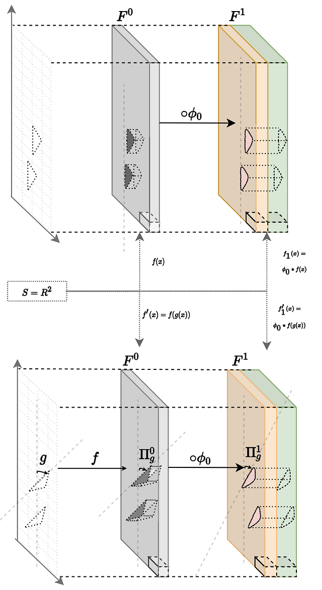
Fig3A: Visual example of equivariant CNN filter. Given the transformation g acting on S and the consequent rotation of the input signal f given by Π₀(g), f1 is rotated by Π1(g).
2.1 Formalization of the problem
We can state that a CNN of n layers is equivariant with respect to a group of transformations G if, for every g in G,0: when an input function f ₀ is transformed to Π₀(g), then the output function of the n-th layer is transformed to a transformation Πn(g).
A sufficient condition to make this statement true is that each contiguous layer is equivariant to transformations on it’s immediate inputs (see fig 3A). The equivariance of the network comes by induction. Following the definitions given in the second article, a filter Φ is equivariant if it satisfies the following condition:

Eq.0: Definition of equivariance
It is now possible to claim the main result of the steerable neural network theory.


Eq.1: Necessary and Sufficient condition for equivariance of a kernel with respect to a transformation g.
In the broader literature [2,3] kernels that adhere to this constraint are called g-steerable kernels. As the kernel constraint operates in a linear manner, the solutions it generates constitute a linear subspace within the vector space of unconstrained kernels typically utilized in standard CNN. Upon closer examination, this definition closely aligns with the concept of steerable filters introduced in paragraph 2 of the last article here. In practical terms, to get this work we need a basis for this kernel subspace, denoted as {k_1, …k_D} , which adheres to Eq.1 . The size of this basis, denoted as D, can be calculated as D = cʿⁿ ʾ ˟ cʿⁿ⁺¹ʾ. The kernel k(x) is subsequently derived through a linear combination of this basis, with the network learning the weights in the process:
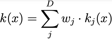
Eq.2: The linearity of Eq(1) makes the solution be equal to the following linear combination.
In a training scenario, our approach involves setting the sizes of both the input and output layers to specific values, namely cʿⁿ ʾ and cʿⁿ⁺¹. Then, based on the transformations we seek equivariance to, we solve the equation and determine a kernel basis. Subsequently, during the training process, we learn the weights associated with these kernels.
2.2 Solving the equation
The solution of the constrain presented in Eq.1 is from being trivial. It depends on three main elements:
More specifically we can say that the choice of the group G defines the type of the network. Specifically we are mainly interested on the following type of networks:
If we operate in a 2D input domain, we have SO(2), SE(2), and E(2) networks [4]. Conversely, with a 3D input domain, we work with SO(3), SE(3), and E(3) networks[1], and indeed this can be extended to any E space [6].
Extending this work into other spaces and symmetries is an area of ongoing research, an interested reader is encouraged to investigate the fields of mathematical study known as Hilbert spaces and Green’s functions, a discussion of which here is out of the scope of this article.

Fig 3B: Basis of harmonic functions in 2D (left) and in 3D (right). This basis constitutes a basis of steerable equivariant filters in SE(2) and SE(3) networks respectively.
Considering a more filter design scenario, in the image Fig 3C below, we see for example how an SO2 steerable equivariant kernel is built for a input layer f ₀: ℝ²->ℝ³ and an output layer of f₁:ℝ²->ℝ².
The kernel is a function k: ℝ²->ℝ³ˣ². Each single element of the matrix is obtained from a function resulting from the linear weighted combination of the D basis sampled at the position (x₁,x₂) . We see the example above for position x=(1,2).
As follows we will show some simple solutions of this equation considering , S=ℝ² and G as group of rotation transformations impling SO2 networks.
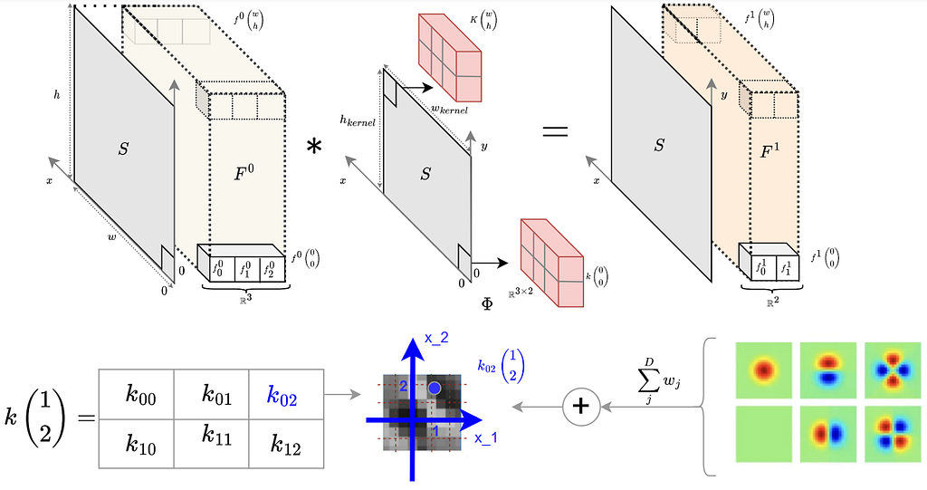
Fig 3C: Visualization representation of a steerable kernel 3x2 is built using a basis of 6 harmonic functions.
2.3 Practical solutions
- Case1A: SO2 networks , k: S=ℝ² → ℝ
Let’s imagine the practical case of having a greyscale image as input and we want to build a steerable filter to process it. First of all, we have to decide the dimension of the output layer (number of features). Let’s take for simplicity dimension 1.
In this setup, we have an input function f: ℝ²-> ℝ and a similar output function f₁: ℝ²-> ℝ. Therefore the kernel function is k: ℝ² -> ℝ. We want our CNN layer to be equivariant to a group of transformations, G, which represents rotations by angle theta within [0,2π) (SO network). For this problem, the kernel function’s basis requires using Eq.1. Given that both f and f¹ are scalar, Pi_out = 1 and Pi_in = 1. This results k[g_θ(x)] = k[x] as written in Eq.3 .
If x = (x₁, x₂) is in ℝ², g(theta) aligns with the 2D Euler matrix.

Eq.3: Rewriting Eq.(1) in case of k: S=ℝ² → ℝ
It is trivial to see that this is solved by each isotropic function in (x₁, x₂) . Specifically this resolves with a one dimensional basis of isotropic (rotation invariant) kernels. (i.e. k(x₁, x₂) = x₁² +x₂²)
Case 2: SO2 filter , k: ℝ² → ℝ²
Let’s take now a more complex case. The input function is f: ℝ² → ℝ² and the output layer is a function f ₁: ℝ² → ℝ². The kernel can be therefore written as function k: S= ℝ² → ℝ² ˣ ²; in other words for each position x in ℝ² we have a bi-dimensional matrix 2x2 (see equation below). We want to build S02 filter so the group of transformations to consider is again G={g(θ)} ={r(θ)} , θ ∈ [0,2Π[. Being ℝ² the codomain of f and f ₁, Π_out=Π_θ and Π_in=Π_θ , where Π_θ is the Euler matrix in ℝ². Considering all these conditions we can rewrite Eq.1 above in the following way:

Eq.(4): kernel function considering k: S= ℝ² → ℝ² ˣ ²

Eq.(5): Rewriting Eq.(1) for a SO2 kernel k: S=ℝ² → ℝ².
For a more comprehensive understanding of the solution to this equation and additional insights, please refer to the appendix section in the paper [4].
2.4 Network non-linearities
So far we have only considered equivariance with respect to the convolution operation, not considering the non-linear part given by the function σ(f(x)): ℝ=ℝ ͨ →ℝ ͨ’ . In session 4.3 of paper [1] and 2.6 session of paper [4] this is widely treated.
Given the function f(x) the condition of equivariance can be summarized as following :

Eq.(5) : Condition of equivariance for the activation function.
As also mentioned in a related YouTube lecture here, it’s possible to create an activation function that meets this criterion by utilizing what’s known as a norm-based activation function like σ(u) = σ(||u||) . The motivation for this is that a scalar norm is transparently invariant and so the application of any nonlinear function to it will result in an invariant output. To prove this, when we apply this formula to the aforementioned condition to Eq.(5) we obtain the following equation:

Eq.(6): Rewriting Eq.(5) as norm-based functions.
If ‘g’ belongs to the group of E transformations, the norm remains constant. Consequently, the equation is universally valid when Π’(g) equals the Identity. This implies that the specially designed activation function is consistently rotation invariant. An example of this , Norm-ReLUs, defined by η(|f(x)|) = ReLU(|f(x)| − b)
Additional nonlinear activation functions have been suggested in the research papers and the lecture, such as non-gated activation functions. We refer the reader to these sources for further explanation.
3) Design a steerable CNN
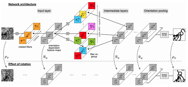
Fig 3D: The architecture of a steerable CNN as described in [3]. Notice the use of the steerable filters in layer 2 coupled together with a G-convolution.
In the previous session, we grasped the fundamentals of constructing a single steerable filter. In this concluding segment, we will delve into the methodology of integrating these filters cohesively to establish a fully-functional steerable neural network.
In the picture above we can see an example taken by the paper [3]. We are particularly interested in layer 2 where the steerable filters are used.
Here, each horizontal representation is a steerable filter — a composite of weighted harmonic functions — that yields a distinct output, denoted as single fⁿ. Observing the structure, it’s apparent that while harmonic functions remain consistent across the filters, their orientations vary from one to the next. This is emblematic of the G-convolution technique, a sophisticated method that contributes to the construction of networks invariant to transformation (you can find more information on this technique here). The network harnesses the power of max-pooling to funnel only the most robust responses from the array of steerable filters into the subsequent layer. This principle of selective transmission ensures that the strongest features are preserved and enhanced as they progress through the network. This approach mirrors the methodologies implemented in other works, such as in reference [5], which successfully crafted a scale-invariant steerable network. The architecture of such a steerable CNN benefits from this technique, as it naturally incorporates scale and rotation invariance, thereby enriching the network’s ability to recognize patterns and features in a more abstract yet robust manner.In any case, it is possible to see from the picture that the final result is a network equivariant to rotations.
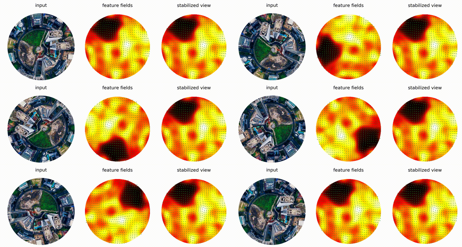
Fig 3E: A visual example of the application of a 2D steerable filter on a rotated image (original can be found here)
An excellent step-by-step explanation about the design of a steerable neural network can be found at this link, included in the Github repo “e2cn” (link). In this repo, it is possible to find the PyTorch code for designing an SE2 steerable network. Useful code for the development of SE3 networks can be found instead at this link, while a quick course on 3D equivariant networks has been published here.
LITERATURE:
[1] “3D Steerable CNNs: Learning Rotationally Equivariant Features in Volumetric Data”, Weilier et al., (link);
[2] “Steerable CNNs”, Cohen et al. ( link);
[3] “Learning Steerable Filters for Rotation Equivariant CNNs”,Weilier et al., (link)
[4] “General E(2)-Equivariant Steerable CNNs” Weilier et al., (link)
[5] “Scale Steerable Filters for the Locally Scale-Invariant Convolutional Neural Network”, Ghosh et al. (link)
[6] “A program to build E -equivariant steerable CNNs.” Cesa et al. (link)
✍️ ?. About the authors:
1️⃣ Matteo Ciprian, Machine Learning Engineer/Researcher
2️⃣ Robert Schoonmaker, Signal Processing/Machine Learning Researcher

A gentle introduction to Steerable Neural Networks (part 2) was originally published in Towards Data Science on Medium, where people are continuing the conversation by highlighting and responding to this story.
1) Introduction
This article is the second and last part of the tutorial “A gentle introduction to Steerable Neural Networks”. It follows the article number one (here).
The first article offers an accessible overview of Steerable Neural Networks (S-CNNs), explaining their purpose and applications. It also delves into the underlying formalism and key concepts, including the definition of equivariance and steerable filters. Although a quick recap of the formalism will be given in the next paragraph, we would recommend you read the first article for a complete understanding.
In this last part of the tutorial, we want to provide a guide on how to build a Steerable Filter and at the end , how to compose a Steerable Neural Network.
Quick recap of nomenclature:
Fig 3A: Representation of a neural network following the formalism.
- S : input domain space. Space where the objects exists (usually ℝ³ or ℝ²).
- f ₙ: a map/function , f ₙ: S → ℝ ͨ ʿⁿ ʾ ( Fₙ) , which describes the n-th feature map of the NN . Note that the f ⁰ is the function describing the input (input layer), while fₙ, with n>0, describe the n-th feature map.
- Fₙ= ℝ ͨ ʿⁿ ʾ, it is codomain of the map f ₙ.
- Φₙ: Fₙ→ F ₙ₊₁, n-th ͑filter of the NN characterizable by the kernel function kⁿ : S → ℝ ͨ ʿⁿ ʾ ˟ ͨ ʿⁿ⁺ ¹ ʾ . The definition of convolution can be seen in the second equation above.
- G: group of transformations ( single element g).
Considering all these concepts we have been able to define convolution as following:


2) Design of a Steerable CNN filter

Fig3A: Visual example of equivariant CNN filter. Given the transformation g acting on S and the consequent rotation of the input signal f given by Π₀(g), f1 is rotated by Π1(g).
2.1 Formalization of the problem
We can state that a CNN of n layers is equivariant with respect to a group of transformations G if, for every g in G,0: when an input function f ₀ is transformed to Π₀(g), then the output function of the n-th layer is transformed to a transformation Πn(g).
A sufficient condition to make this statement true is that each contiguous layer is equivariant to transformations on it’s immediate inputs (see fig 3A). The equivariance of the network comes by induction. Following the definitions given in the second article, a filter Φ is equivariant if it satisfies the following condition:

Eq.0: Definition of equivariance
It is now possible to claim the main result of the steerable neural network theory.
Be k the kernel connecting the layer f ₙwith f such that fₙ₊₁ = k* f ₙ.
The convolution k* f ₙis equivariant with respect to a transformation g, if and only if :

or simpler

Eq.1: Necessary and Sufficient condition for equivariance of a kernel with respect to a transformation g.
In the broader literature [2,3] kernels that adhere to this constraint are called g-steerable kernels. As the kernel constraint operates in a linear manner, the solutions it generates constitute a linear subspace within the vector space of unconstrained kernels typically utilized in standard CNN. Upon closer examination, this definition closely aligns with the concept of steerable filters introduced in paragraph 2 of the last article here. In practical terms, to get this work we need a basis for this kernel subspace, denoted as {k_1, …k_D} , which adheres to Eq.1 . The size of this basis, denoted as D, can be calculated as D = cʿⁿ ʾ ˟ cʿⁿ⁺¹ʾ. The kernel k(x) is subsequently derived through a linear combination of this basis, with the network learning the weights in the process:

Eq.2: The linearity of Eq(1) makes the solution be equal to the following linear combination.
In a training scenario, our approach involves setting the sizes of both the input and output layers to specific values, namely cʿⁿ ʾ and cʿⁿ⁺¹. Then, based on the transformations we seek equivariance to, we solve the equation and determine a kernel basis. Subsequently, during the training process, we learn the weights associated with these kernels.
2.2 Solving the equation
The solution of the constrain presented in Eq.1 is from being trivial. It depends on three main elements:
- the space S, whether it is S= ℝ³ or S= ℝ².
- The group G.
- The input out dimension of the layers: cʿⁿ ʾ and cʿⁿ⁺ ¹ ʾ.
More specifically we can say that the choice of the group G defines the type of the network. Specifically we are mainly interested on the following type of networks:
- SO Networks: Equivariant to rotations in the Special Orthogonal Group (SO).
- SE Networks: Equivariant to rotations and translations within the Special Euclidean Group (SE).
- E Networks: Equivariant to rotations, translations, and reflections in the Euclidean Group (E).
If we operate in a 2D input domain, we have SO(2), SE(2), and E(2) networks [4]. Conversely, with a 3D input domain, we work with SO(3), SE(3), and E(3) networks[1], and indeed this can be extended to any E
Extending this work into other spaces and symmetries is an area of ongoing research, an interested reader is encouraged to investigate the fields of mathematical study known as Hilbert spaces and Green’s functions, a discussion of which here is out of the scope of this article.
However it is possible to see that in case of SE networks the general solution of Eq.1 is a harmonic basis function in S= ℝⁿ. In the image above (Fig 3B) it is possible the harmonic functions in ℝ² on the left and harmonic functions in ℝ³.

Fig 3B: Basis of harmonic functions in 2D (left) and in 3D (right). This basis constitutes a basis of steerable equivariant filters in SE(2) and SE(3) networks respectively.
Considering a more filter design scenario, in the image Fig 3C below, we see for example how an SO2 steerable equivariant kernel is built for a input layer f ₀: ℝ²->ℝ³ and an output layer of f₁:ℝ²->ℝ².
The kernel is a function k: ℝ²->ℝ³ˣ². Each single element of the matrix is obtained from a function resulting from the linear weighted combination of the D basis sampled at the position (x₁,x₂) . We see the example above for position x=(1,2).
As follows we will show some simple solutions of this equation considering , S=ℝ² and G as group of rotation transformations impling SO2 networks.

Fig 3C: Visualization representation of a steerable kernel 3x2 is built using a basis of 6 harmonic functions.
2.3 Practical solutions
- Case1A: SO2 networks , k: S=ℝ² → ℝ
Let’s imagine the practical case of having a greyscale image as input and we want to build a steerable filter to process it. First of all, we have to decide the dimension of the output layer (number of features). Let’s take for simplicity dimension 1.
In this setup, we have an input function f: ℝ²-> ℝ and a similar output function f₁: ℝ²-> ℝ. Therefore the kernel function is k: ℝ² -> ℝ. We want our CNN layer to be equivariant to a group of transformations, G, which represents rotations by angle theta within [0,2π) (SO network). For this problem, the kernel function’s basis requires using Eq.1. Given that both f and f¹ are scalar, Pi_out = 1 and Pi_in = 1. This results k[g_θ(x)] = k[x] as written in Eq.3 .
If x = (x₁, x₂) is in ℝ², g(theta) aligns with the 2D Euler matrix.

Eq.3: Rewriting Eq.(1) in case of k: S=ℝ² → ℝ
It is trivial to see that this is solved by each isotropic function in (x₁, x₂) . Specifically this resolves with a one dimensional basis of isotropic (rotation invariant) kernels. (i.e. k(x₁, x₂) = x₁² +x₂²)
Case 2: SO2 filter , k: ℝ² → ℝ²
Let’s take now a more complex case. The input function is f: ℝ² → ℝ² and the output layer is a function f ₁: ℝ² → ℝ². The kernel can be therefore written as function k: S= ℝ² → ℝ² ˣ ²; in other words for each position x in ℝ² we have a bi-dimensional matrix 2x2 (see equation below). We want to build S02 filter so the group of transformations to consider is again G={g(θ)} ={r(θ)} , θ ∈ [0,2Π[. Being ℝ² the codomain of f and f ₁, Π_out=Π_θ and Π_in=Π_θ , where Π_θ is the Euler matrix in ℝ². Considering all these conditions we can rewrite Eq.1 above in the following way:

Eq.(4): kernel function considering k: S= ℝ² → ℝ² ˣ ²

Eq.(5): Rewriting Eq.(1) for a SO2 kernel k: S=ℝ² → ℝ².
For a more comprehensive understanding of the solution to this equation and additional insights, please refer to the appendix section in the paper [4].
2.4 Network non-linearities
So far we have only considered equivariance with respect to the convolution operation, not considering the non-linear part given by the function σ(f(x)): ℝ=ℝ ͨ →ℝ ͨ’ . In session 4.3 of paper [1] and 2.6 session of paper [4] this is widely treated.
Given the function f(x) the condition of equivariance can be summarized as following :

Eq.(5) : Condition of equivariance for the activation function.
As also mentioned in a related YouTube lecture here, it’s possible to create an activation function that meets this criterion by utilizing what’s known as a norm-based activation function like σ(u) = σ(||u||) . The motivation for this is that a scalar norm is transparently invariant and so the application of any nonlinear function to it will result in an invariant output. To prove this, when we apply this formula to the aforementioned condition to Eq.(5) we obtain the following equation:

Eq.(6): Rewriting Eq.(5) as norm-based functions.
If ‘g’ belongs to the group of E transformations, the norm remains constant. Consequently, the equation is universally valid when Π’(g) equals the Identity. This implies that the specially designed activation function is consistently rotation invariant. An example of this , Norm-ReLUs, defined by η(|f(x)|) = ReLU(|f(x)| − b)
Additional nonlinear activation functions have been suggested in the research papers and the lecture, such as non-gated activation functions. We refer the reader to these sources for further explanation.
3) Design a steerable CNN

Fig 3D: The architecture of a steerable CNN as described in [3]. Notice the use of the steerable filters in layer 2 coupled together with a G-convolution.
In the previous session, we grasped the fundamentals of constructing a single steerable filter. In this concluding segment, we will delve into the methodology of integrating these filters cohesively to establish a fully-functional steerable neural network.
In the picture above we can see an example taken by the paper [3]. We are particularly interested in layer 2 where the steerable filters are used.
Here, each horizontal representation is a steerable filter — a composite of weighted harmonic functions — that yields a distinct output, denoted as single fⁿ. Observing the structure, it’s apparent that while harmonic functions remain consistent across the filters, their orientations vary from one to the next. This is emblematic of the G-convolution technique, a sophisticated method that contributes to the construction of networks invariant to transformation (you can find more information on this technique here). The network harnesses the power of max-pooling to funnel only the most robust responses from the array of steerable filters into the subsequent layer. This principle of selective transmission ensures that the strongest features are preserved and enhanced as they progress through the network. This approach mirrors the methodologies implemented in other works, such as in reference [5], which successfully crafted a scale-invariant steerable network. The architecture of such a steerable CNN benefits from this technique, as it naturally incorporates scale and rotation invariance, thereby enriching the network’s ability to recognize patterns and features in a more abstract yet robust manner.In any case, it is possible to see from the picture that the final result is a network equivariant to rotations.

Fig 3E: A visual example of the application of a 2D steerable filter on a rotated image (original can be found here)
An excellent step-by-step explanation about the design of a steerable neural network can be found at this link, included in the Github repo “e2cn” (link). In this repo, it is possible to find the PyTorch code for designing an SE2 steerable network. Useful code for the development of SE3 networks can be found instead at this link, while a quick course on 3D equivariant networks has been published here.
LITERATURE:
[1] “3D Steerable CNNs: Learning Rotationally Equivariant Features in Volumetric Data”, Weilier et al., (link);
[2] “Steerable CNNs”, Cohen et al. ( link);
[3] “Learning Steerable Filters for Rotation Equivariant CNNs”,Weilier et al., (link)
[4] “General E(2)-Equivariant Steerable CNNs” Weilier et al., (link)
[5] “Scale Steerable Filters for the Locally Scale-Invariant Convolutional Neural Network”, Ghosh et al. (link)
[6] “A program to build E
✍️ ?. About the authors:
1️⃣ Matteo Ciprian, Machine Learning Engineer/Researcher
- MSc in Telecommunications Engineering at University of Padua. Currently working in the field of Sensor Fusion, Signal Processing and applied AI. Experience in projects related to AI applications in eHealth and wearable technologies (academic research and corporate domains). Specialized in developing Anomaly Detection algorithms, as well as advancing techniques in Deep Learning and Sensor Fusion.
Passionate about Philosophy. Content creator in Youtube.
? Links:
? Linkedin
? Youtube
??Instagram
2️⃣ Robert Schoonmaker, Signal Processing/Machine Learning Researcher
- PhD in Computational Condensed Matter Physics from Durham University. Specializes in applied machine learning and nonlinear statistics, currently investigating the uses of GPU compute methods on synthetic aperture radar and similar systems. Experience includes developing symmetric ML methods for use in sensor fusion and positioning techniques.
? Links:
? Linkedin
A gentle introduction to Steerable Neural Networks (part 2) was originally published in Towards Data Science on Medium, where people are continuing the conversation by highlighting and responding to this story.
