Here’s how to tackle chaotic problems using math, physics, Python and data science

Image by author generated using Midjourney
Three years ago I moved from Rome, Italy and I started living in Cincinnati, Ohio, USA, after a PhD offer from University of Cincinnati. There were (and there are) a lot of things that I miss about my city: the food, the weather, the beauty of the eternal city. One thing that I absolutely don’t miss about my city is the insane traffic.
A good friend of mine texted me the other day and said
Now, obviously, I didn’t correct him (especially knowing how the traffic is in Rome), but the term chaos has a totally different meaning in math and physics with respect to how we use “chaos” in our everyday lives.
A popular definition of chaos, when we refer to chaos in math, is the one of a problem that is regulated by deterministic equations, but the evolution of the system is extremely dependent on the original conditions. This means that even with an extremely small change in the original conditions, the evolution of the system can be incredibly different. To say it in the words of Lorentz¹ this means that:
¹ http://mpe.dimacs.rutgers.edu/2013/03/17/chaos-in-an-atmosphere-hanging-on-a-wall/
This means that the only way that we are able to predict the evolution of a state is by considering it from a probabilistic point of view.
Given the starting point of a process, we won’t be able to predict exactly the arrival point of the system, as it’s chaotic, but we will be able to predict it probabilistically, in the sense that we will be able to get, for example, the mean and start deviation.
This kind of chaos can be treated numerically, for example using Python. In this blog post, we will describe the Polynomial Chaos Expansion (PCE) starting from the abstract Random Walk to the application on a real case with our coffee temperature ☕️
Let’s get started!
1. Random Walk
The random walk is something that is well known to all the mathematicians and the physicists who are reading. This model has been used pretty much everywhere, from finance to physics, and it is very simple. It is also known in the literature as Brownian motion and it works like this:
For once, I think that the pseudocode is even more easy to understand than explaining it in words
RandomWalk(N):
x = 0
i = 0
while i<N:
p = random(-1,1)
x = x+p
i = i+1
return x
Now let’s explore this, shall we?
1.2 Code
In this part of the post, we will describe the Random Walk using the Python language code. You will need to import very basic libraries like numpy and matplotlib.pyplot.
This is the Random Walk code:
If we run this, let’s say 100 times we get the following paths:
What’s very interesting is that you can find the gaussian distribution if you consider the last step:
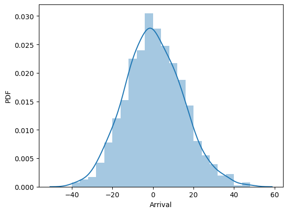
Let’s leave it here for now. I promise, we will use this.
2. Differential Equations
Now, all we know about life, wait, literally, all we know about life we know it because of the differential equation.
The differential equations are the tools that physics use to describe the evolution of a system. My high school teacher explained it by saying:
For example, let’s consider the location y of a squirrel climbing on the tree:

Image by author generated using Midjourney
Let’s say that the speed of the squirrel is v(t) = (t/60)**2, where t = seconds. So our superhero start with a v(t=0) = 0 and after two minutes he gets to the speed v(120) = 2**2 = 4 m/s .
Given this information, what is the location of the super-squirrel?
What we need to do is to integrate the velocity equation and we get:

How do we get that c constant? We just set what happens at t = 0. We assume that our squirrel starts at height = 0 so c = 0.
So the location of our super squirrel that climbs the tree is the following:
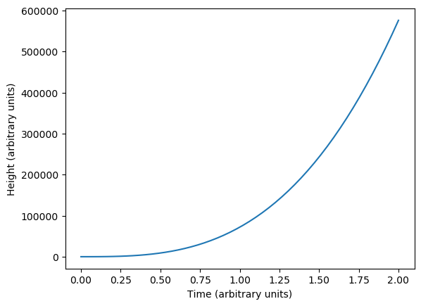
In general, a certain solution y can be seen as an integration of another quantity, say xand a starting condition.
In this scheme we talked about:
So in this case we can say that x (t) = integration of y(t).
There is more. You can have some parameters in your system that are fixed but that can change the evolution of your system. So:
x(t, list of parameters) = integration of y(t, list of parameters)
For example. Let’s talk about coffee. Coffee? , coffee.
2.1 Newton’s law of cooling
A guy that was pretty decent in Physics (lol) named Isaac Netwon, among the many gifts he left us, explained how to describe the heat transfer of a hot body. In other words, he told us how things cool down

Image by author generated using Midjourney
The law of cooling proposed by Newton states that the rate of heat from the body to the outside is proportional to a constant k that is dependent on the surface area and its heat transfer coefficient and the difference between the temperature T at time t and the temperature of the environment T_env.
If we want to get the temperature (T), we need to integrate the rate of heat (dT/dt).
This is the equation:

Image by author
To get the temperature T, given T_env and k (remember this!!!), we need to integrate dT/dt.
3. Wiener’s Chaos!
Rarely, very rarely, we are able to define an analytical solution for the differential equation. That is why my high school professor said that it’s very hard to integrate. We are more likely in need of doing a numerical integration, which means solving the differential equation in a numerical way (a.k.a. with an algorithm).
There are super well-known methods (algorithms) for integrations, like the trapezoidal or the Riemann sum. They work, with their pros and cons, and they work efficiently. They are not the problem.
The real problem is in the parameters (e.g. T_env and kappa) of the differential equation. Let me elaborate.
Do you remember T_env and k from the equation above? We have no idea of what they might actually be, and it can completely change the evolution of our system.
The beautiful mind of Norbert Wiener made a very elegant formulation of the differential equations with additional random parameters. In particular, and now all our talk makes sense, the differential equations with random parameters are defined as chaotic and can be described using random walks (ah-ha!) as a polynomial. By doing this, we are able to understand the solution T(t) in a probabilistic way!
I understand it can be confusing: let’s do it step by step
3.1 The setup
The first thing that we need, in Python, is to define our differential equation:
As we see, it’s not only a matter of T (our variable) but a matter of kappa and T_env too.
This is the function that we need to integrate. Before doing that, let’s import some friends ?♂️
You will probably have an error cause you don’t have chaospy and uncertainpy. Those are our magic wizards: they implement the polynomial chaos expansion method. It’s super easy to install them:
pip install uncertainpy
3.2 Integrating the function
Let’s set up the function to integrate using the trapezoidal rule:
So:
Now, I have to say this: uncertainpy is awesome. There are so many things you can do with it and I really recommend you to spend some time on it here.
What we are going to do is the following:
The game is easy: if we know the possible distribution of the parameters thanks to the Wiener’s chaos we are able to know the distribution of the output.
It might sound confusing but I swear it’s going to be more clear after showing you the code:
The model is defined with the coffee_cup, which is our differential equation. We then define the parameter distributions (using chaospy) and define the corresponding parameters dictionary.
Now. For each value of kappa and T_env we have a differential equation with different parameters and different Temperatures T(t), that are the result of integration. Thanks to the use of the magic chaospy the solutions become a distribution with mean and std.
Let’s see how:
That’s that! (like Biggie). So easy.
3.4 The whole thing
The whole thing can be put in this single block of code:
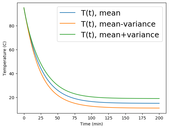
Isn’t this beautiful? We are able to convert the distribution of the parameters in the input in the distribution of the result of the output. At time t=0, the temperature is the T= T_0 = 95. When the time increases, the uncertainty in the parameters become more and more present. We have a big uncertainty (let’s say from 5 to 30) at Time = 200 minutes, it could be cold or a little bit hot depending on k and T_env.
4. Results
In this blog post, we described the beautiful chaospy and uncertainpy libraries. These libraries allowed us to treat the Wiener Chaos problem, which uses the Random Walk to define a form of polynomial chaos. This polynomial chaos is used to treat differential equations with distributions instead of parameters. We did this in the following order:
If you liked the article and you want to know more about machine learning, or you just want to ask me something, you can:
A. Follow me on Linkedin, where I publish all my stories
B. Subscribe to my newsletter. It will keep you updated about new stories and give you the chance to text me to receive all the corrections or doubts you may have.
C. Become a referred member, so you won’t have any “maximum number of stories for the month” and you can read whatever I (and thousands of other Machine Learning and Data Science top writers) write about the newest technology available.

Finding Order in Chaos with Polynomial Chaos Expansion, using uncertainpy and chaospy was originally published in Towards Data Science on Medium, where people are continuing the conversation by highlighting and responding to this story.

Image by author generated using Midjourney
Three years ago I moved from Rome, Italy and I started living in Cincinnati, Ohio, USA, after a PhD offer from University of Cincinnati. There were (and there are) a lot of things that I miss about my city: the food, the weather, the beauty of the eternal city. One thing that I absolutely don’t miss about my city is the insane traffic.
A good friend of mine texted me the other day and said
“Piero, today the traffic is so bad and the city is a total chaos”.
Now, obviously, I didn’t correct him (especially knowing how the traffic is in Rome), but the term chaos has a totally different meaning in math and physics with respect to how we use “chaos” in our everyday lives.
A popular definition of chaos, when we refer to chaos in math, is the one of a problem that is regulated by deterministic equations, but the evolution of the system is extremely dependent on the original conditions. This means that even with an extremely small change in the original conditions, the evolution of the system can be incredibly different. To say it in the words of Lorentz¹ this means that:
“The present determines the future, but the approximate present does not approximately determine the future.”
¹ http://mpe.dimacs.rutgers.edu/2013/03/17/chaos-in-an-atmosphere-hanging-on-a-wall/
This means that the only way that we are able to predict the evolution of a state is by considering it from a probabilistic point of view.
Given the starting point of a process, we won’t be able to predict exactly the arrival point of the system, as it’s chaotic, but we will be able to predict it probabilistically, in the sense that we will be able to get, for example, the mean and start deviation.
This kind of chaos can be treated numerically, for example using Python. In this blog post, we will describe the Polynomial Chaos Expansion (PCE) starting from the abstract Random Walk to the application on a real case with our coffee temperature ☕️
Let’s get started!
1. Random Walk
The random walk is something that is well known to all the mathematicians and the physicists who are reading. This model has been used pretty much everywhere, from finance to physics, and it is very simple. It is also known in the literature as Brownian motion and it works like this:
- We start from a point x = 0
- With the same probability we can go from x=0 to x=1 or from x=0 to x=-1. We define this point as x_1
- Again, we can increase the value of x_1 by +1 or -1. We will define this point x_2.
- We repeat point 3 with x_2 for N-2 more times
For once, I think that the pseudocode is even more easy to understand than explaining it in words
RandomWalk(N):
x = 0
i = 0
while i<N:
p = random(-1,1)
x = x+p
i = i+1
return x
Now let’s explore this, shall we?
1.2 Code
In this part of the post, we will describe the Random Walk using the Python language code. You will need to import very basic libraries like numpy and matplotlib.pyplot.
This is the Random Walk code:
If we run this, let’s say 100 times we get the following paths:
What’s very interesting is that you can find the gaussian distribution if you consider the last step:

Let’s leave it here for now. I promise, we will use this.
2. Differential Equations
Now, all we know about life, wait, literally, all we know about life we know it because of the differential equation.
The differential equations are the tools that physics use to describe the evolution of a system. My high school teacher explained it by saying:
“To describe the world you need two things: to differentiate and to integrate. It’s very easy to differentiate, it’s very hard to integrate.”
For example, let’s consider the location y of a squirrel climbing on the tree:

Image by author generated using Midjourney
Let’s say that the speed of the squirrel is v(t) = (t/60)**2, where t = seconds. So our superhero start with a v(t=0) = 0 and after two minutes he gets to the speed v(120) = 2**2 = 4 m/s .
Given this information, what is the location of the super-squirrel?
What we need to do is to integrate the velocity equation and we get:

How do we get that c constant? We just set what happens at t = 0. We assume that our squirrel starts at height = 0 so c = 0.
So the location of our super squirrel that climbs the tree is the following:

In general, a certain solution y can be seen as an integration of another quantity, say xand a starting condition.
In this scheme we talked about:
- The time (t) that is the time variable (that goes from the start to the end of the experiment)
- x, that is the object that we are integrating (in the example above x is the velocity)
- The solution (y) that is the solution that we obtain integrating x (in the example above y is the location of the super squirrel)
So in this case we can say that x (t) = integration of y(t).
There is more. You can have some parameters in your system that are fixed but that can change the evolution of your system. So:
x(t, list of parameters) = integration of y(t, list of parameters)
For example. Let’s talk about coffee. Coffee?
 , coffee.
2.1 Newton’s law of cooling
A guy that was pretty decent in Physics (lol) named Isaac Netwon, among the many gifts he left us, explained how to describe the heat transfer of a hot body. In other words, he told us how things cool down

Image by author generated using Midjourney
The law of cooling proposed by Newton states that the rate of heat from the body to the outside is proportional to a constant k that is dependent on the surface area and its heat transfer coefficient and the difference between the temperature T at time t and the temperature of the environment T_env.
If we want to get the temperature (T), we need to integrate the rate of heat (dT/dt).
This is the equation:

Image by author
To get the temperature T, given T_env and k (remember this!!!), we need to integrate dT/dt.
3. Wiener’s Chaos!
Rarely, very rarely, we are able to define an analytical solution for the differential equation. That is why my high school professor said that it’s very hard to integrate. We are more likely in need of doing a numerical integration, which means solving the differential equation in a numerical way (a.k.a. with an algorithm).
There are super well-known methods (algorithms) for integrations, like the trapezoidal or the Riemann sum. They work, with their pros and cons, and they work efficiently. They are not the problem.
The real problem is in the parameters (e.g. T_env and kappa) of the differential equation. Let me elaborate.
Do you remember T_env and k from the equation above? We have no idea of what they might actually be, and it can completely change the evolution of our system.
The beautiful mind of Norbert Wiener made a very elegant formulation of the differential equations with additional random parameters. In particular, and now all our talk makes sense, the differential equations with random parameters are defined as chaotic and can be described using random walks (ah-ha!) as a polynomial. By doing this, we are able to understand the solution T(t) in a probabilistic way!
I understand it can be confusing: let’s do it step by step
3.1 The setup
The first thing that we need, in Python, is to define our differential equation:
As we see, it’s not only a matter of T (our variable) but a matter of kappa and T_env too.
This is the function that we need to integrate. Before doing that, let’s import some friends ?♂️
You will probably have an error cause you don’t have chaospy and uncertainpy. Those are our magic wizards: they implement the polynomial chaos expansion method. It’s super easy to install them:
pip install uncertainpy
3.2 Integrating the function
Let’s set up the function to integrate using the trapezoidal rule:
So:
- We set the starting temperature of our coffee, let’s say T_0 = 95
- We set the time step of our problem, let’s say 500 time steps
- We integrate it using the trapezoidal rule
- We return the time and temperature
Now, I have to say this: uncertainpy is awesome. There are so many things you can do with it and I really recommend you to spend some time on it here.
What we are going to do is the following:
- We set a distribution of possible kappas. For example, kappa is sampled from a normal distribution with a given mu and variance.
- We do the same with T_env
- We apply uncertainpy and extract a distribution of possible values of Temperature given the input distributions
The game is easy: if we know the possible distribution of the parameters thanks to the Wiener’s chaos we are able to know the distribution of the output.
It might sound confusing but I swear it’s going to be more clear after showing you the code:
The model is defined with the coffee_cup, which is our differential equation. We then define the parameter distributions (using chaospy) and define the corresponding parameters dictionary.
Now. For each value of kappa and T_env we have a differential equation with different parameters and different Temperatures T(t), that are the result of integration. Thanks to the use of the magic chaospy the solutions become a distribution with mean and std.
Let’s see how:
That’s that! (like Biggie). So easy.
3.4 The whole thing
The whole thing can be put in this single block of code:

Isn’t this beautiful? We are able to convert the distribution of the parameters in the input in the distribution of the result of the output. At time t=0, the temperature is the T= T_0 = 95. When the time increases, the uncertainty in the parameters become more and more present. We have a big uncertainty (let’s say from 5 to 30) at Time = 200 minutes, it could be cold or a little bit hot depending on k and T_env.
4. Results
In this blog post, we described the beautiful chaospy and uncertainpy libraries. These libraries allowed us to treat the Wiener Chaos problem, which uses the Random Walk to define a form of polynomial chaos. This polynomial chaos is used to treat differential equations with distributions instead of parameters. We did this in the following order:
- We described the random walk in Chapter 1.
- We described differential equations in Chapter 2. In particular we described the Netwon Cooling Law.
- We described chaos according to Wiener and applied the polynomial chaos in Chapter 3.
If you liked the article and you want to know more about machine learning, or you just want to ask me something, you can:
A. Follow me on Linkedin, where I publish all my stories
B. Subscribe to my newsletter. It will keep you updated about new stories and give you the chance to text me to receive all the corrections or doubts you may have.
C. Become a referred member, so you won’t have any “maximum number of stories for the month” and you can read whatever I (and thousands of other Machine Learning and Data Science top writers) write about the newest technology available.
Finding Order in Chaos with Polynomial Chaos Expansion, using uncertainpy and chaospy was originally published in Towards Data Science on Medium, where people are continuing the conversation by highlighting and responding to this story.
