A concrete case study
SHAP (SHapley Additive exPlanations) values are designed to fairly allocate the contribution of each feature to the prediction made by a machine learning model, based on the concept of Shapley values from cooperative game theory. The Shapley value framework has several desirable theoretical properties and can, in principle, handle any predictive model. However, SHAP values can potentially be misleading, especially when using the KernelSHAP method for approximation. When predictors are correlated, these approximations can be imprecise and even have the opposite sign.
In this blog post, I will demonstrate how the original SHAP values can differ significantly from approximations made by the SHAP framework, especially the KernalSHAP and discuss the reasons behind these discrepancies.
Case Study: Churn Rate
Consider a scenario where we aim to predict the churn rate of rental leases in an office building, based on two key factors: occupancy rate and the rate of reported problems.
The occupancy rate significantly impacts the churn rate. For instance, if the occupancy rate is too low, tenants may leave due to the office being underutilized. Conversely, if the occupancy rate is too high, tenants might depart because of overcrowding, seeking better options elsewhere.
Furthermore, let’s assume that the rate of reported problems is highly correlated with the occupancy rate, specifically that the reported problem rate is the square of the occupancy rate.
We define the churn rate function as follows:

Image by author: churn rate function
This function with respect to the two variables can be represented by the following illustrations:
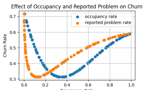
Image by author: Churn on two variables
Discrepancies between original SHAP and Kernel SHAP
SHAP Values Computed Using Kernel SHAP
We will now use the following code to compute the SHAP values of the predictors:
# Define the dataframe
churn_df=pd.DataFrame(
{
"occupancy_rate":occupancy_rates,
"reported_problem_rate": reported_problem_rates,
"churn_rate":churn_rates,
}
)
X=churn_df.drop(["churn_rate"],axis=1)
y=churn_df["churn_rate"]
X_train, X_test, y_train, y_test = train_test_split(X, y, test_size=0.2, random_state = 42)
# append one speical point
X_test=pd.concat(objs=[X_test, pd.DataFrame({"occupancy_rate":[0.8], "reported_problem_rate":[0.64]})])
# Define the prediction
def predict_fn(data):
occupancy_rates = data[:, 0]
reported_problem_rates = data[:, 1]
churn_rate= C_base +C_churn*(C_occ* occupancy_rates-reported_problem_rates-0.6)**2 +C_problem*reported_problem_rates
return churn_rate
# Create the SHAP KernelExplainer using the correct prediction function
background_data = shap.sample(X_train,100)
explainer = shap.KernelExplainer(predict_fn, background_data)
shap_values = explainer(X_test)
The code above performs the following tasks:
Below, you can see a summary SHAP bar plot, which represents the average SHAP values for X_test :
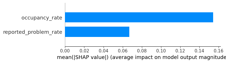
Image by author: average shap values
In particular, we see that at the data point (0.8, 0.64), the SHAP values of the two features are 0.10 and -0.03, illustrated by the following force plot:
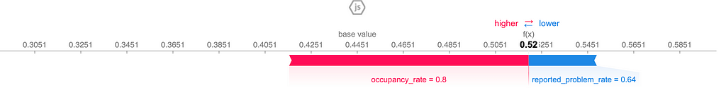
Image by author Force Plot of one data point
SHAP Values by orignal definition
Let’s take a step back and compute the exact SHAP values step by step according to their original definition. The general formula for SHAP values is given by:

where: S is a subset of all feature indices excluding i, |S| is the size of the subset S, M is the total number of features, f(XS∪{xi}) is the function evaluated with the features in S with xi present while f(XS) is the function evaluated with the feature in S with xi absent.
Now, let’s calculate the SHAP values for two features: occupancy rate (denoted as x1x_1x1) and reported problem rate (denoted as x2x_2x2) at the data point (0.8, 0.64). Recall that x1x_1x1 and x2x_2x2 are related by x_1 = x_2².
We have the SHAP value for occupancy rate at the data point:

and, similary, for the feature reported problem rate:

First, let’s compute the SHAP value for the occupancy rate at the data point:
Thus, the SHAP values compute from the original definition for the two features occupancy rate and reported problem rate at the data point (0.8, 0.64) are -0.0375 and -0.0375, respectively, which is quite different from the values given by Kernel SHAP.
Where comes discrepancies?
Cause of Discrepancies in SHAP Values
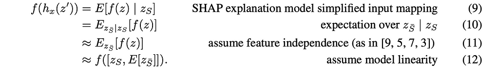
As you may have noticed, the discrepancy between the two methods primarily arises from the second and fourth steps, where we need to compute the conditional expectation. This involves calculating the expectation of the model’s output when X1X_1X1 is conditioned on 0.8.
Screenshot from the paper
Potential resolutions
Unfortunately, computing SHAP values directly based on their original definition can be computationally expensive. Here are some alternative approaches to consider:
TreeSHAP
By utilizing these methods, you can address the computational challenges associated with calculating SHAP values and enhance their accuracy in practical applications. However, it is important to note that no single solution is universally optimal for all scenarios.
Conclusion
In this blog post, we’ve explored how SHAP values, despite their strong theoretical foundation and versatility across various predictive models, can suffer from accuracy issues when predictors are correlated, particularly when approximations like KernelSHAP are employed. Understanding these limitations is crucial for effectively interpreting SHAP values. By recognizing the potential discrepancies and selecting the most suitable approximation methods, we can achieve more accurate and reliable feature attribution in our models.

KernelSHAP can be misleading with correlated predictors was originally published in Towards Data Science on Medium, where people are continuing the conversation by highlighting and responding to this story.
“Like many other permutation-based interpretation methods, the Shapley value method suffers from inclusion of unrealistic data instances when features are correlated. To simulate that a feature value is missing from a coalition, we marginalize the feature. ..When features are dependent, then we might sample feature values that do not make sense for this instance. ”— Interpretable-ML-Book.
SHAP (SHapley Additive exPlanations) values are designed to fairly allocate the contribution of each feature to the prediction made by a machine learning model, based on the concept of Shapley values from cooperative game theory. The Shapley value framework has several desirable theoretical properties and can, in principle, handle any predictive model. However, SHAP values can potentially be misleading, especially when using the KernelSHAP method for approximation. When predictors are correlated, these approximations can be imprecise and even have the opposite sign.
In this blog post, I will demonstrate how the original SHAP values can differ significantly from approximations made by the SHAP framework, especially the KernalSHAP and discuss the reasons behind these discrepancies.
Case Study: Churn Rate
Consider a scenario where we aim to predict the churn rate of rental leases in an office building, based on two key factors: occupancy rate and the rate of reported problems.
The occupancy rate significantly impacts the churn rate. For instance, if the occupancy rate is too low, tenants may leave due to the office being underutilized. Conversely, if the occupancy rate is too high, tenants might depart because of overcrowding, seeking better options elsewhere.
Furthermore, let’s assume that the rate of reported problems is highly correlated with the occupancy rate, specifically that the reported problem rate is the square of the occupancy rate.
We define the churn rate function as follows:
Image by author: churn rate function
This function with respect to the two variables can be represented by the following illustrations:
Image by author: Churn on two variables
Discrepancies between original SHAP and Kernel SHAP
SHAP Values Computed Using Kernel SHAP
We will now use the following code to compute the SHAP values of the predictors:
# Define the dataframe
churn_df=pd.DataFrame(
{
"occupancy_rate":occupancy_rates,
"reported_problem_rate": reported_problem_rates,
"churn_rate":churn_rates,
}
)
X=churn_df.drop(["churn_rate"],axis=1)
y=churn_df["churn_rate"]
X_train, X_test, y_train, y_test = train_test_split(X, y, test_size=0.2, random_state = 42)
# append one speical point
X_test=pd.concat(objs=[X_test, pd.DataFrame({"occupancy_rate":[0.8], "reported_problem_rate":[0.64]})])
# Define the prediction
def predict_fn(data):
occupancy_rates = data[:, 0]
reported_problem_rates = data[:, 1]
churn_rate= C_base +C_churn*(C_occ* occupancy_rates-reported_problem_rates-0.6)**2 +C_problem*reported_problem_rates
return churn_rate
# Create the SHAP KernelExplainer using the correct prediction function
background_data = shap.sample(X_train,100)
explainer = shap.KernelExplainer(predict_fn, background_data)
shap_values = explainer(X_test)
The code above performs the following tasks:
- Data Preparation: A DataFrame named churn_df is created with columns occupancy_rate, reported_problem_rate, and churn_rate. Variables and target (churn_rate ) are then created from and Data is split into training and testing sets, with 80% for training and 20% for testing. Note that a special data point with specific occupancy_rate and reported_problem_rate values is added to the test set X_test.
- Prediction Function Definition: A function predict_fn is defined to calculate churn rate using a specific formula involving predefined constants.
- SHAP Analysis: A SHAP KernelExplainer is initialized using the prediction function and background_data samples from X_train. SHAP values for X_test are computed using the explainer.
Below, you can see a summary SHAP bar plot, which represents the average SHAP values for X_test :
Image by author: average shap values
In particular, we see that at the data point (0.8, 0.64), the SHAP values of the two features are 0.10 and -0.03, illustrated by the following force plot:
Image by author Force Plot of one data point
SHAP Values by orignal definition
Let’s take a step back and compute the exact SHAP values step by step according to their original definition. The general formula for SHAP values is given by:
where: S is a subset of all feature indices excluding i, |S| is the size of the subset S, M is the total number of features, f(XS∪{xi}) is the function evaluated with the features in S with xi present while f(XS) is the function evaluated with the feature in S with xi absent.
Now, let’s calculate the SHAP values for two features: occupancy rate (denoted as x1x_1x1) and reported problem rate (denoted as x2x_2x2) at the data point (0.8, 0.64). Recall that x1x_1x1 and x2x_2x2 are related by x_1 = x_2².
We have the SHAP value for occupancy rate at the data point:
and, similary, for the feature reported problem rate:
First, let’s compute the SHAP value for the occupancy rate at the data point:
- The first term is the expectation of the model’s output when X1 is fixed at 0.8 and X2 is averaged over its distribution. Given the relationship xx_1 = x_2², this expectation leads to the model’s output at the specific point (0.8, 0.64).
- The second term is the unconditional expectation of the model’s output, where both X1 and X2 are averaged over their distributions. This can be computed by averaging the outputs over all data points in the background dataset.
- The third term is the model’s output at the specific point (0.8, 0.64).
- The final term is the expectation of the model’s output when X1 is averaged over its distribution, given that X2 is fixed at the specific point 0.64. Again, due to the relationship x_1 = x_2², this expectation matches the model’s output at (0.8, 0.64), similar to the first step.
Thus, the SHAP values compute from the original definition for the two features occupancy rate and reported problem rate at the data point (0.8, 0.64) are -0.0375 and -0.0375, respectively, which is quite different from the values given by Kernel SHAP.
Where comes discrepancies?
Cause of Discrepancies in SHAP Values
As you may have noticed, the discrepancy between the two methods primarily arises from the second and fourth steps, where we need to compute the conditional expectation. This involves calculating the expectation of the model’s output when X1X_1X1 is conditioned on 0.8.
- Exact SHAP: When computing exact SHAP values, the dependencies between features (such as x1=x_2² in our example) are explicitly accounted for. This ensures accurate calculations by considering how feature interactions impact the model’s output.
- Kernel SHAP: By default, Kernel SHAP assumes feature independence, which can lead to inaccurate SHAP values when features are actually dependent. According to the paper A Unified Approach to Interpreting Model Predictions, this assumption is a simplification. In practice, features are often correlated, making it challenging to achieve accurate approximations when using Kernel SHAP.
Screenshot from the paper
Potential resolutions
Unfortunately, computing SHAP values directly based on their original definition can be computationally expensive. Here are some alternative approaches to consider:
TreeSHAP
- Designed specifically for tree-based models like random forests and gradient boosting machines, TreeSHAP efficiently computes SHAP values while effectively managing feature dependencies.
- This method is optimized for tree ensembles, making it faster and more scalable compared to traditional SHAP computations.
- When using TreeSHAP within the SHAP framework, set the parameter feature_perturbation = "interventional" to account for feature dependencies accurately.
- To address feature dependencies, this paper involves extending Kernel SHAP. One method is to assume that the feature vector follows a multivariate Gaussian distribution. In this approach:
- Conditional distributions are modeled as multivariate Gaussian distributions.
- Samples are generated from these conditional Gaussian distributions using estimates from the training data.
- The integral in the approximation is computed based on these samples.
- This method assumes a multivariate Gaussian distribution for features, which may not always be applicable in real-world scenarios where features can exhibit different dependency structures.
- Description: Enhance the accuracy of Kernel SHAP by ensuring that the background dataset used for approximation is representative of the actual data distribution with independant features.
By utilizing these methods, you can address the computational challenges associated with calculating SHAP values and enhance their accuracy in practical applications. However, it is important to note that no single solution is universally optimal for all scenarios.
Conclusion
In this blog post, we’ve explored how SHAP values, despite their strong theoretical foundation and versatility across various predictive models, can suffer from accuracy issues when predictors are correlated, particularly when approximations like KernelSHAP are employed. Understanding these limitations is crucial for effectively interpreting SHAP values. By recognizing the potential discrepancies and selecting the most suitable approximation methods, we can achieve more accurate and reliable feature attribution in our models.
KernelSHAP can be misleading with correlated predictors was originally published in Towards Data Science on Medium, where people are continuing the conversation by highlighting and responding to this story.