Not All HNSW Indices Are Made Equally
Overcoming Major HNSW Challenges to Improve the Efficiency of Your AI Production Workload

Photo by Talha Riaz on Pexels
The Hierarchical Navigable Small World (HNSW) algorithm is known for its efficiency and accuracy in high-scale data searches, making it a popular choice for search tasks and AI/LLM applications like RAG. However, setting up and maintaining an HNSW index comes with its own set of challenges. Let’s explore these challenges, offer some ways to overcome them, and even see how we can kill two birds with one stone by addressing just one of them.
Memory Consumption
Due to its hierarchical structure of embeddings, one of the primary challenges of HNSW is its high memory usage. But not many realize that the memory issue extends beyond the memory required to store the initial index. This is because, as an HNSW index is modified, the memory required to store nodes and their connections increases even more. This will be explained in greater depth in a later section. Memory awareness is important since the more memory you need for your data, the longer it will take to compute (search) over it, and the more expensive it will get to maintain your workload.
Build Time

Photo by Andrea De Santis on Unsplash
In the process of creating an index, nodes are added to the graph according to how close they are to other nodes on the graph. For every node, a dynamic list of its closest neighbors is kept at each level of the graph. This process involves iterating over the list and performing similarity searches to determine if a node’s neighbors are closer to the query. This computationally heavy iterative process significantly increases the overall build time of the index, negatively impacting your users’ experience and costing you more in cloud usage expenses.
Parameter Tuning
HNSW requires predefined configuration parameters in it’s build process. Optimizing HNSW those parameters: M (the number of connections per node), and ef_construction (the size of the dynamic list for the nearest neighbors which is used during the index construction) is crucial for balancing search speed, accuracy and the use of memory. Incorrect parameter settings can lead to poor performance and increased production costs. Fine-tuning these parameters is unique for every index and is a continuous process that requires often re-building of indices.
Rebuilding Indices

Photo by Robin Jonathan Deutsch on Unsplash
Rebuilding an HNSW index is one of the most resource-intensive aspects of using HNSW in production workloads. Unlike traditional databases, where data deletions can be handled by simply deleting a row in a table, using HNSW in a vector database often requires a complete rebuild to maintain optimal performance and accuracy.
Why is Rebuilding Necessary?
Because of its layered graph structure, HNSW is not inherently designed for dynamic datasets that change frequently. Adding new data or deleting existing data is essential for maintaining updated data, especially for use cases like RAG, which aims to improve search relevence.
Most databases work on a concept called “hard” and “soft” deletes. Hard deletes permanently remove data, while soft deletes flag data as ‘to-be-deleted’ and remove it later. The issue with soft deletes is that the to-be-deleted data still uses significant memory until it is permanently removed. This is particularly problematic in vector databases that use HNSW, where memory consumption is already a significant issue.
HNSW creates a graph where nodes (vectors) are connected based on their proximity in the vector space, and traversing on an HNSW graph is done like a skip-list. In order to support that, the layers of the graph are designed so that some layers have very few nodes. When vectors are deleted, especially those on layers that have very few nodes that serve as critical connectors in the graph, the whole HNSW structure can become fragmented. This fragmentation may lead to nodes (or layers) that are disconnected from the main graph, which require rebuilding of the entire graph, or at the very least will result in a degradation in the efficiency of searches.
HNSW then uses a soft-delete technique, which marks vectors for deletion but does not immediately remove them. This approach lowers the expense of frequent complete rebuilds, although periodic reconstruction is still needed to maintain the graph’s optimal state.
Addressing HNSW Challenges
So what ways do we have to manage those challenges? Here are a few that worked for me:
A 2-D vector space example (for simplicity). Image by the author.
2. Frequent index rebuilds — One way to overcome the HNSW expanding memory challenge is to frequently rebuild your index so that you get rid of nodes that are marked as “to-be-deleted”, which take up space and reduce search speed. Consider making a copy of your index during those times so you don’t suffer complete downtime (However, this will require a lot of memory — an already big issue with HNSW).
3. Parallel Index Build — Building an index in parallel involves partitioning the data and the allocated memory and distributing the indexing process across multiple CPU cores. In this process, all operations are mapped to available RAM. For instance, a system might partition the data into manageable chunks, assign each chunk to a different processor core, and have them build their respective parts of the index simultaneously. This parallelization allows for better utilization of the system’s resources, resulting in faster index creation times, especially for large datasets. This is a faster way to build indices compared to traditional single-threaded builds; however, challenges arise when the entire index cannot fit into memory or when a CPU does not have enough cores to support your workload in the required timeframe.
Parallel Processing. Image by the author.
Using Custom Build Accelerators: A Different Approach
While the above strategies can help, they often require significant expertise and development. Introducing GXL, a new paid-for tool designed to enhance HNSW index construction. It uses the APU, GSI Technology’s compute-in-memory Associative Processing Unit, which uses its millions of bit processors to perform computation within the memory. This architecture enables massive parallel processing of nearest neighbor distance calculations, significantly accelerating index build times for large-scale dynamic datasets. It uses a custom algorithm that combines vector quantization and overcomes the similarity search bottleneck with parallalism using unique hardware to reduce the overall index build time.
Let’s check out some benchmark numbers:
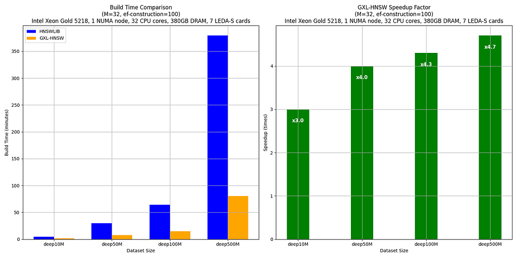
Image by the author. Credit: Ron Bar Hen
The benchmarks compare the build times of HNSWLIB and GXL-HNSW for various dataset sizes (deep10M, deep50M, deep100M, and deep500M — all subsets of deep1B) using the parameters M = 32 and ef-construction = 100. These tests were conducted on a server with an Intel(R) Xeon(R) Gold 5218 CPU @ 2.30GHz, using one NUMA node (32 CPU cores, 380GB DRAM, and 7 LEDA-S APU cards).
The results clearly show that GXL-HNSW significantly outperforms HNSWLIB across all dataset sizes. For instance, GXL-HNSW builds the deep10M dataset in 1 minute and 35 seconds, while HNSWLIB takes 4 minutes and 44 seconds, demonstrating a speedup factor of 3.0. As the dataset size increases, the efficiency of GXL-HNSW becomes even greater, with speedup factors of 4.0 for deep50M, 4.3 for deep100M, and 4.7 for deep500M. This consistent improvement highlights GXL-HNSW’s better performance in handling large-scale data, making it a more efficient choice for large-scale dataset similarity searches.
In conclusion, while HNSW is highly effective for vector search and AI pipelines, it faces tough challenges such as slow index building times and high memory usage, which becomes even greater because of HNSW’s complex deletion management. Strategies to address these challenges include optimizing your memory usage through frequent index rebuilding, implementing vector quantization to your index, and parallelizing your index construction. GXL offers an approach that effectively combines some of these strategies. These methods help maintain accuracy and efficiency in systems relying on HNSW. By reducing the time it takes to build indices, index rebuilding isn’t as much of a time-intensive issue as it once was, enableing us to kill two birds with one stone — solving both the memory expansion problem and long index building times. Test out which method suits you best, and I hope this helps improve your overall production workload performance.

Not All HNSW Indices Are Made Equaly was originally published in Towards Data Science on Medium, where people are continuing the conversation by highlighting and responding to this story.
Overcoming Major HNSW Challenges to Improve the Efficiency of Your AI Production Workload
Photo by Talha Riaz on Pexels
The Hierarchical Navigable Small World (HNSW) algorithm is known for its efficiency and accuracy in high-scale data searches, making it a popular choice for search tasks and AI/LLM applications like RAG. However, setting up and maintaining an HNSW index comes with its own set of challenges. Let’s explore these challenges, offer some ways to overcome them, and even see how we can kill two birds with one stone by addressing just one of them.
Memory Consumption
Due to its hierarchical structure of embeddings, one of the primary challenges of HNSW is its high memory usage. But not many realize that the memory issue extends beyond the memory required to store the initial index. This is because, as an HNSW index is modified, the memory required to store nodes and their connections increases even more. This will be explained in greater depth in a later section. Memory awareness is important since the more memory you need for your data, the longer it will take to compute (search) over it, and the more expensive it will get to maintain your workload.
Build Time
Photo by Andrea De Santis on Unsplash
In the process of creating an index, nodes are added to the graph according to how close they are to other nodes on the graph. For every node, a dynamic list of its closest neighbors is kept at each level of the graph. This process involves iterating over the list and performing similarity searches to determine if a node’s neighbors are closer to the query. This computationally heavy iterative process significantly increases the overall build time of the index, negatively impacting your users’ experience and costing you more in cloud usage expenses.
Parameter Tuning
HNSW requires predefined configuration parameters in it’s build process. Optimizing HNSW those parameters: M (the number of connections per node), and ef_construction (the size of the dynamic list for the nearest neighbors which is used during the index construction) is crucial for balancing search speed, accuracy and the use of memory. Incorrect parameter settings can lead to poor performance and increased production costs. Fine-tuning these parameters is unique for every index and is a continuous process that requires often re-building of indices.
Rebuilding Indices
Photo by Robin Jonathan Deutsch on Unsplash
Rebuilding an HNSW index is one of the most resource-intensive aspects of using HNSW in production workloads. Unlike traditional databases, where data deletions can be handled by simply deleting a row in a table, using HNSW in a vector database often requires a complete rebuild to maintain optimal performance and accuracy.
Why is Rebuilding Necessary?
Because of its layered graph structure, HNSW is not inherently designed for dynamic datasets that change frequently. Adding new data or deleting existing data is essential for maintaining updated data, especially for use cases like RAG, which aims to improve search relevence.
Most databases work on a concept called “hard” and “soft” deletes. Hard deletes permanently remove data, while soft deletes flag data as ‘to-be-deleted’ and remove it later. The issue with soft deletes is that the to-be-deleted data still uses significant memory until it is permanently removed. This is particularly problematic in vector databases that use HNSW, where memory consumption is already a significant issue.
HNSW creates a graph where nodes (vectors) are connected based on their proximity in the vector space, and traversing on an HNSW graph is done like a skip-list. In order to support that, the layers of the graph are designed so that some layers have very few nodes. When vectors are deleted, especially those on layers that have very few nodes that serve as critical connectors in the graph, the whole HNSW structure can become fragmented. This fragmentation may lead to nodes (or layers) that are disconnected from the main graph, which require rebuilding of the entire graph, or at the very least will result in a degradation in the efficiency of searches.
HNSW then uses a soft-delete technique, which marks vectors for deletion but does not immediately remove them. This approach lowers the expense of frequent complete rebuilds, although periodic reconstruction is still needed to maintain the graph’s optimal state.
Addressing HNSW Challenges
So what ways do we have to manage those challenges? Here are a few that worked for me:
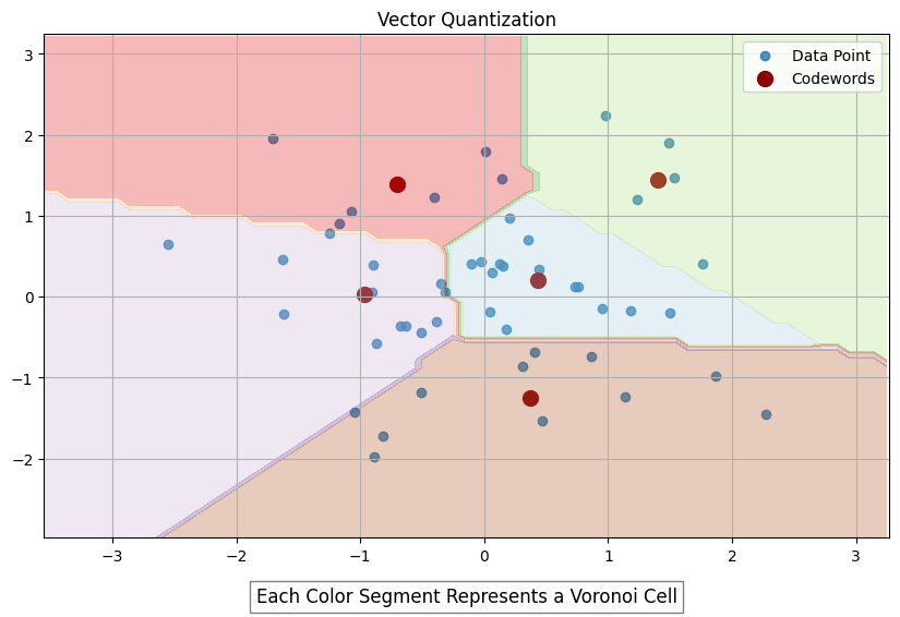
- Vector Quantization — Vector quantization (VQ) is a process that maps k-dimensional vectors from a vector space ℝ^k into a finite set of vectors known as codewords (for example, by using the Linde-Buzo-Gray (LBG) algorithm), which form a codebook. Each codeword Yi has an associated region called a Voronoi region, which partitions the entire space ℝ^k into regions based on proximity to the codewords (see graph below). When an input vector is provided, it is compared with each codeword in the codebook to find the closest match. This is done by identifying the codeword in the codebook with the minimum Euclidean distance to the input vector. Instead of transmitting or storing the entire input vector, the index of the nearest codeword is sent (encoding). When retrieving the vector (decoding), the decoder retrieves the corresponding codeword from the codebook. The codeword is used as an approximation of the original input vector. The reconstructed vector is an approximation of the original data, but it typically retains the most significant characteristics due to the nature of the VQ process. VQ is one popular way to reduce index build time and the amount of memory used to store the HNSW graph. However, it is important to understand that it will also reduce the accuracy of your search results.
A 2-D vector space example (for simplicity). Image by the author.
2. Frequent index rebuilds — One way to overcome the HNSW expanding memory challenge is to frequently rebuild your index so that you get rid of nodes that are marked as “to-be-deleted”, which take up space and reduce search speed. Consider making a copy of your index during those times so you don’t suffer complete downtime (However, this will require a lot of memory — an already big issue with HNSW).
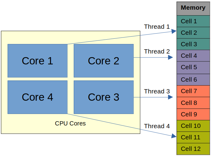
3. Parallel Index Build — Building an index in parallel involves partitioning the data and the allocated memory and distributing the indexing process across multiple CPU cores. In this process, all operations are mapped to available RAM. For instance, a system might partition the data into manageable chunks, assign each chunk to a different processor core, and have them build their respective parts of the index simultaneously. This parallelization allows for better utilization of the system’s resources, resulting in faster index creation times, especially for large datasets. This is a faster way to build indices compared to traditional single-threaded builds; however, challenges arise when the entire index cannot fit into memory or when a CPU does not have enough cores to support your workload in the required timeframe.
Parallel Processing. Image by the author.
Using Custom Build Accelerators: A Different Approach
While the above strategies can help, they often require significant expertise and development. Introducing GXL, a new paid-for tool designed to enhance HNSW index construction. It uses the APU, GSI Technology’s compute-in-memory Associative Processing Unit, which uses its millions of bit processors to perform computation within the memory. This architecture enables massive parallel processing of nearest neighbor distance calculations, significantly accelerating index build times for large-scale dynamic datasets. It uses a custom algorithm that combines vector quantization and overcomes the similarity search bottleneck with parallalism using unique hardware to reduce the overall index build time.
Let’s check out some benchmark numbers:
Image by the author. Credit: Ron Bar Hen
The benchmarks compare the build times of HNSWLIB and GXL-HNSW for various dataset sizes (deep10M, deep50M, deep100M, and deep500M — all subsets of deep1B) using the parameters M = 32 and ef-construction = 100. These tests were conducted on a server with an Intel(R) Xeon(R) Gold 5218 CPU @ 2.30GHz, using one NUMA node (32 CPU cores, 380GB DRAM, and 7 LEDA-S APU cards).
The results clearly show that GXL-HNSW significantly outperforms HNSWLIB across all dataset sizes. For instance, GXL-HNSW builds the deep10M dataset in 1 minute and 35 seconds, while HNSWLIB takes 4 minutes and 44 seconds, demonstrating a speedup factor of 3.0. As the dataset size increases, the efficiency of GXL-HNSW becomes even greater, with speedup factors of 4.0 for deep50M, 4.3 for deep100M, and 4.7 for deep500M. This consistent improvement highlights GXL-HNSW’s better performance in handling large-scale data, making it a more efficient choice for large-scale dataset similarity searches.
In conclusion, while HNSW is highly effective for vector search and AI pipelines, it faces tough challenges such as slow index building times and high memory usage, which becomes even greater because of HNSW’s complex deletion management. Strategies to address these challenges include optimizing your memory usage through frequent index rebuilding, implementing vector quantization to your index, and parallelizing your index construction. GXL offers an approach that effectively combines some of these strategies. These methods help maintain accuracy and efficiency in systems relying on HNSW. By reducing the time it takes to build indices, index rebuilding isn’t as much of a time-intensive issue as it once was, enableing us to kill two birds with one stone — solving both the memory expansion problem and long index building times. Test out which method suits you best, and I hope this helps improve your overall production workload performance.
Not All HNSW Indices Are Made Equaly was originally published in Towards Data Science on Medium, where people are continuing the conversation by highlighting and responding to this story.