The Magic of Mixture Density Networks Explained
Tired of your neural networks making lame predictions? 🤦♂️ Wish they could predict more than just the average future? Enter Mixture Density Networks (MDNs), a supercharged approach that doesn’t just guess the future — it predicts a whole spectrum of possibilities!
When trying to predict the future but all you see are Gaussian curves.
A Blast from the Past
Christopher M. Bishop’s 1994 paper, Mixture Density Networks¹, is where the magic began. It’s a classic! 📚 Bishop basically said, “Why settle for one guess when you can have a whole bunch of them?” And thus, MDNs were born.
MDNs: The Sorcerers of Uncertainty
MDNs take your boring old neural network and turn it into a prediction powerhouse. Why settle for one prediction when you can have an entire buffet of potential outcomes?
If life throws complex, unpredictable scenarios your way, MDNs are ready with a probability-laden safety net.
The Core Idea
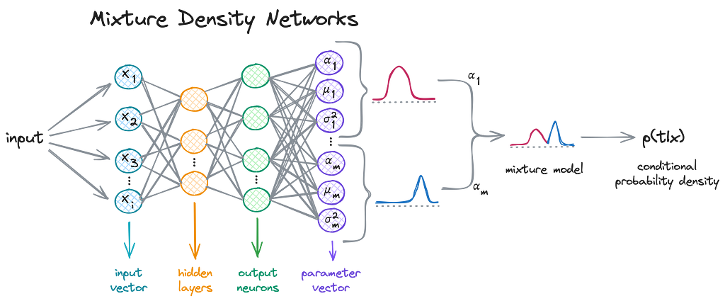
In a MDN, the probability density of the target variable t given the input x is represented as a linear combination of kernel functions, typically Gaussian functions, though not limited to. In math speak:

Where 𝛼ᵢ(x) are the mixing coefficients, and who doesn’t love a good mix, am I right? 🎛️ These determine how much weight each component 𝜙ᵢ(t|x) — each Gaussian in our case — holds in the model.
Brewing the Gaussians ☕
Each Gaussian component 𝜙ᵢ(t|x) has its own mean 𝜇ᵢ(x) and variance 𝜎ᵢ².

Mixing It Up 🎧 with Coefficients
The mixing coefficients 𝛼ᵢ are crucial as they balance the influence of each Gaussian component, governed by a softmax function to ensure they sum up to 1:

Magical Parameters ✨ Means & Variances
Means 𝜇ᵢ and variances 𝜎ᵢ² define each Gaussian. And guess what? Variances have to be positive! We achieve this by using the exponential of the network outputs:

Training Our Wizardry 🧙♀️
Alright, so how do we train this beast? Well, it’s all about maximizing the likelihood of our observed data. Fancy terms, I know. Let’s see it in action.
The Log-Likelihood Spell ✨
The likelihood of our data under the MDN model is the product of the probabilities assigned to each data point. In math speak:

This basically says, “Hey, what’s the chance we got this data given our model?”. But products can get messy, so we take the log (because math loves logs), which turns our product into a sum:

Now, here’s the kicker: we actually want to minimize the negative log likelihood because our optimization algorithms like to minimize things. So, plugging in the definition of p(t|x), the error function we actually minimize is:

This formula might look intimidating, but it’s just saying we sum up the log probabilities across all data points, then throw in a negative sign because minimization is our jam.
From Math to Magic in Code 🧑💻
Now here’s how to translate our wizardry into Python, and you can find the full code here:
GitHub - pandego/mdn-playground: A playground for Mixture Density Networks.
The Loss Function
def mdn_loss(alpha, sigma, mu, target, eps=1e-8):
target = target.unsqueeze(1).expand_as(mu)
m = torch.distributions.Normal(loc=mu, scale=sigma)
log_prob = m.log_prob(target)
log_prob = log_prob.sum(dim=2)
log_alpha = torch.log(alpha + eps) # Avoid log(0) disaster
loss = -torch.logsumexp(log_alpha + log_prob, dim=1)
return loss.mean()
Here’s the breakdown:
Let’s create a neural network that’s all set to handle the wizardry:
class MDN(nn.Module):
def __init__(self, input_dim, output_dim, num_hidden, num_mixtures):
super(MDN, self).__init__()
self.hidden = nn.Sequential(
nn.Linear(input_dim, num_hidden),
nn.Tanh(),
nn.Linear(num_hidden, num_hidden),
nn.Tanh(),
)
self.z_alpha = nn.Linear(num_hidden, num_mixtures)
self.z_sigma = nn.Linear(num_hidden, num_mixtures * output_dim)
self.z_mu = nn.Linear(num_hidden, num_mixtures * output_dim)
self.num_mixtures = num_mixtures
self.output_dim = output_dim
def forward(self, x):
hidden = self.hidden(x)
alpha = F.softmax(self.z_alpha(hidden), dim=-1)
sigma = torch.exp(self.z_sigma(hidden)).view(-1, self.num_mixtures, self.output_dim)
mu = self.z_mu(hidden).view(-1, self.num_mixtures, self.output_dim)
return alpha, sigma, mu
Notice the softmax being applied to 𝛼ᵢ alpha = F.softmax(self.z_alpha(hidden), dim=-1), so they sum up to 1, and the exponential to 𝜎ᵢ sigma = torch.exp(self.z_sigma(hidden)).view(-1, self.num_mixtures, self.output_dim), to ensure they remain positive, as explained earlier.
The Prediction
Getting predictions from MDNs is a bit of a trick. Here’s how you sample from the mixture model:
def get_sample_preds(alpha, sigma, mu, samples=10):
N, K, T = mu.shape
sampled_preds = torch.zeros(N, samples, T)
uniform_samples = torch.rand(N, samples)
cum_alpha = alpha.cumsum(dim=1)
for i, j in itertools.product(range(N), range(samples)):
u = uniform_samples[i, j]
k = torch.searchsorted(cum_alpha, u).item()
sampled_preds[i, j] = torch.normal(mu[i, k], sigma[i, k])
return sampled_preds
Here’s the breakdown:
Practical Example: Predicting the ‘Apparent’ 🌡️
Let’s apply MDNs to predict ‘Apparent Temperature’ using a simple Weather Dataset. I trained an MDN with a 50-hidden-layer network, and guess what? It rocks! 🎸
Find the full code here. Here are some results:
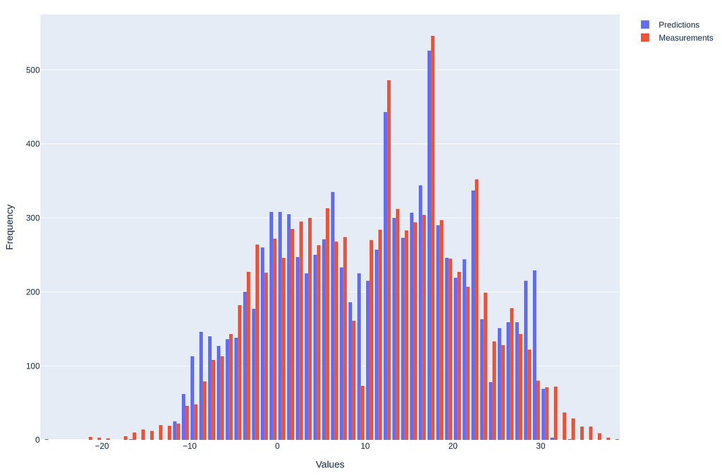
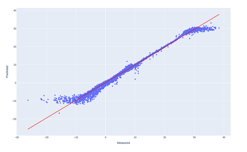
Histogram (left) and Scatterplot (right) of ‘Apparent Temperature’, Measured vs Predictions (R² = .99 and MAE = .5).
The results are pretty sweet, and with some hyper-parameter tuning and data preprocessing, for instance outliers removal and resampling, it could be even better!
The Future is Multimodal 🎆
Consider a scenario where data exhibits a complex pattern, such as a dataset from financial markets or biometric readings. Linear regression would struggle here, capturing none of the underlying dynamics. Non-linear regression might contour to the data better but still falls short in quantifying the uncertainty or capturing multiple potential outcomes. MDNs leap beyond, offering a comprehensive model that anticipates various possibilities, each with its own likelihood!
Embrace the Chaos!
These neural network wizards excel in predicting chaotic, complex scenarios where traditional models just fall flat. Stock market predictions, guessing the weather, or foreseeing the next viral meme 🦄 — MDNs have got you covered.
MDNs are Awesome!
But MDNs don’t just predict — they give you a range of possible futures. They’re your crystal ball 🔮 for understanding uncertainty, capturing intricate relationships, and providing a probabilistic peek into what lies ahead. For researchers, practitioners, or AI enthusiasts, MDNs are a fascinating frontier in the vast, wondrous realm of machine learning!
References
[1] Christopher M. Bishop, Mixture Density Networks (1994), Neural Computing Research Group Report.
Unless otherwise noted, all images are by the author.

Predicting the Unpredictable 🔮 was originally published in Towards Data Science on Medium, where people are continuing the conversation by highlighting and responding to this story.
Tired of your neural networks making lame predictions? 🤦♂️ Wish they could predict more than just the average future? Enter Mixture Density Networks (MDNs), a supercharged approach that doesn’t just guess the future — it predicts a whole spectrum of possibilities!
When trying to predict the future but all you see are Gaussian curves.
A Blast from the Past
Christopher M. Bishop’s 1994 paper, Mixture Density Networks¹, is where the magic began. It’s a classic! 📚 Bishop basically said, “Why settle for one guess when you can have a whole bunch of them?” And thus, MDNs were born.
MDNs: The Sorcerers of Uncertainty
MDNs take your boring old neural network and turn it into a prediction powerhouse. Why settle for one prediction when you can have an entire buffet of potential outcomes?
If life throws complex, unpredictable scenarios your way, MDNs are ready with a probability-laden safety net.
The Core Idea
In a MDN, the probability density of the target variable t given the input x is represented as a linear combination of kernel functions, typically Gaussian functions, though not limited to. In math speak:
Where 𝛼ᵢ(x) are the mixing coefficients, and who doesn’t love a good mix, am I right? 🎛️ These determine how much weight each component 𝜙ᵢ(t|x) — each Gaussian in our case — holds in the model.
Brewing the Gaussians ☕
Each Gaussian component 𝜙ᵢ(t|x) has its own mean 𝜇ᵢ(x) and variance 𝜎ᵢ².
Mixing It Up 🎧 with Coefficients
The mixing coefficients 𝛼ᵢ are crucial as they balance the influence of each Gaussian component, governed by a softmax function to ensure they sum up to 1:
Magical Parameters ✨ Means & Variances
Means 𝜇ᵢ and variances 𝜎ᵢ² define each Gaussian. And guess what? Variances have to be positive! We achieve this by using the exponential of the network outputs:
Training Our Wizardry 🧙♀️
Alright, so how do we train this beast? Well, it’s all about maximizing the likelihood of our observed data. Fancy terms, I know. Let’s see it in action.
The Log-Likelihood Spell ✨
The likelihood of our data under the MDN model is the product of the probabilities assigned to each data point. In math speak:
This basically says, “Hey, what’s the chance we got this data given our model?”. But products can get messy, so we take the log (because math loves logs), which turns our product into a sum:
Now, here’s the kicker: we actually want to minimize the negative log likelihood because our optimization algorithms like to minimize things. So, plugging in the definition of p(t|x), the error function we actually minimize is:
This formula might look intimidating, but it’s just saying we sum up the log probabilities across all data points, then throw in a negative sign because minimization is our jam.
From Math to Magic in Code 🧑💻
Now here’s how to translate our wizardry into Python, and you can find the full code here:
GitHub - pandego/mdn-playground: A playground for Mixture Density Networks.
The Loss Function
def mdn_loss(alpha, sigma, mu, target, eps=1e-8):
target = target.unsqueeze(1).expand_as(mu)
m = torch.distributions.Normal(loc=mu, scale=sigma)
log_prob = m.log_prob(target)
log_prob = log_prob.sum(dim=2)
log_alpha = torch.log(alpha + eps) # Avoid log(0) disaster
loss = -torch.logsumexp(log_alpha + log_prob, dim=1)
return loss.mean()
Here’s the breakdown:
- target = target.unsqueeze(1).expand_as(mu): Expand the target to match the shape of mu.
- m = torch.distributions.Normal(loc=mu, scale=sigma): Create a normal distribution.
- log_prob = m.log_prob(target): Calculate the log probability.
- log_prob = log_prob.sum(dim=2): Sum log probabilities.
- log_alpha = torch.log(alpha + eps): Calculate log of mixing coefficients.
- loss = -torch.logsumexp(log_alpha + log_prob, dim=1): Combine and log-sum-exp the probabilities.
- return loss.mean(): Return the average loss.
Let’s create a neural network that’s all set to handle the wizardry:
class MDN(nn.Module):
def __init__(self, input_dim, output_dim, num_hidden, num_mixtures):
super(MDN, self).__init__()
self.hidden = nn.Sequential(
nn.Linear(input_dim, num_hidden),
nn.Tanh(),
nn.Linear(num_hidden, num_hidden),
nn.Tanh(),
)
self.z_alpha = nn.Linear(num_hidden, num_mixtures)
self.z_sigma = nn.Linear(num_hidden, num_mixtures * output_dim)
self.z_mu = nn.Linear(num_hidden, num_mixtures * output_dim)
self.num_mixtures = num_mixtures
self.output_dim = output_dim
def forward(self, x):
hidden = self.hidden(x)
alpha = F.softmax(self.z_alpha(hidden), dim=-1)
sigma = torch.exp(self.z_sigma(hidden)).view(-1, self.num_mixtures, self.output_dim)
mu = self.z_mu(hidden).view(-1, self.num_mixtures, self.output_dim)
return alpha, sigma, mu
Notice the softmax being applied to 𝛼ᵢ alpha = F.softmax(self.z_alpha(hidden), dim=-1), so they sum up to 1, and the exponential to 𝜎ᵢ sigma = torch.exp(self.z_sigma(hidden)).view(-1, self.num_mixtures, self.output_dim), to ensure they remain positive, as explained earlier.
The Prediction
Getting predictions from MDNs is a bit of a trick. Here’s how you sample from the mixture model:
def get_sample_preds(alpha, sigma, mu, samples=10):
N, K, T = mu.shape
sampled_preds = torch.zeros(N, samples, T)
uniform_samples = torch.rand(N, samples)
cum_alpha = alpha.cumsum(dim=1)
for i, j in itertools.product(range(N), range(samples)):
u = uniform_samples[i, j]
k = torch.searchsorted(cum_alpha, u).item()
sampled_preds[i, j] = torch.normal(mu[i, k], sigma[i, k])
return sampled_preds
Here’s the breakdown:
- N, K, T = mu.shape: Get the number of data points, mixture components, and output dimensions.
- sampled_preds = torch.zeros(N, samples, T): Initialize the tensor to store sampled predictions.
- uniform_samples = torch.rand(N, samples): Generate uniform random numbers for sampling.
- cum_alpha = alpha.cumsum(dim=1): Compute the cumulative sum of mixture weights.
- for i, j in itertools.product(range(N), range(samples)): Loop over each combination of data points and samples.
- u = uniform_samples[i, j]: Get a random number for the current sample.
- k = torch.searchsorted(cum_alpha, u).item(): Find the mixture component index.
[*]sampled_preds[i, j] = torch.normal(mu[i, k], sigma[i, k]): Sample from the selected Gaussian component.
[*]return sampled_preds: Return the tensor of sampled predictions.
Practical Example: Predicting the ‘Apparent’ 🌡️
Let’s apply MDNs to predict ‘Apparent Temperature’ using a simple Weather Dataset. I trained an MDN with a 50-hidden-layer network, and guess what? It rocks! 🎸
Find the full code here. Here are some results:
Histogram (left) and Scatterplot (right) of ‘Apparent Temperature’, Measured vs Predictions (R² = .99 and MAE = .5).
The results are pretty sweet, and with some hyper-parameter tuning and data preprocessing, for instance outliers removal and resampling, it could be even better!
The Future is Multimodal 🎆
Consider a scenario where data exhibits a complex pattern, such as a dataset from financial markets or biometric readings. Linear regression would struggle here, capturing none of the underlying dynamics. Non-linear regression might contour to the data better but still falls short in quantifying the uncertainty or capturing multiple potential outcomes. MDNs leap beyond, offering a comprehensive model that anticipates various possibilities, each with its own likelihood!
Embrace the Chaos!
These neural network wizards excel in predicting chaotic, complex scenarios where traditional models just fall flat. Stock market predictions, guessing the weather, or foreseeing the next viral meme 🦄 — MDNs have got you covered.
MDNs are Awesome!
But MDNs don’t just predict — they give you a range of possible futures. They’re your crystal ball 🔮 for understanding uncertainty, capturing intricate relationships, and providing a probabilistic peek into what lies ahead. For researchers, practitioners, or AI enthusiasts, MDNs are a fascinating frontier in the vast, wondrous realm of machine learning!
References
[1] Christopher M. Bishop, Mixture Density Networks (1994), Neural Computing Research Group Report.
Unless otherwise noted, all images are by the author.
Predicting the Unpredictable 🔮 was originally published in Towards Data Science on Medium, where people are continuing the conversation by highlighting and responding to this story.