Enhancing linear methods by smartly incorporating state features into the learning objective
Reinforcement learning is a domain in machine learning that introduces the concept of an agent learning optimal strategies in complex environments. The agent learns from its actions, which result in rewards, based on the environment’s state. Reinforcement learning is a challenging topic and differs significantly from other areas of machine learning.
What is remarkable about reinforcement learning is that the same algorithms can be used to enable the agent adapt to completely different, unknown, and complex conditions.
About this article
In part 7, we introduced value-function approximation algorithms which scale standard tabular methods. Apart from that, we particularly focused on a very important case when the approximated value function is linear. As we found out, the linearity provides guaranteed convergence either to the global optimum or to the TD fixed point (in semi-gradient methods).
The problem is that sometimes we might want to use a more complex approximation value function, rather than just a simple scalar product, without leaving the linear optimization space. The motivation behind using complex approximation functions is the fact that they fail to account for any information of interaction between features. Since the true state values might have a very sophisticated functional dependency on the input features, their simple linear form might not be enough for good approximation.
In this article, we will understand how to efficiently inject more valuable information about state features into the objective without leaving the linear optimization space.
Reinforcement Learning
Idea
Problem
Imagine a state vector containing features related to the state:

As we know, this vector is multiplied by the weight vector w, which we would like to find:

Due to the linearity constraint, we cannot simply include other terms containing interactions between coefficients of w. For instance, adding the term w₁w₂ makes the optimization problem quadratic:

For semi-gradient methods, we do not know how to optimize such objectives.
Solution
If you remember the previous part, you know that we can include any information about the state into the feature vector x(s). So if we want to add interaction between features into the objective, why not simply derive new features containing that information?
Let us return to the maze example in the previous article. As a reminder, we originally had two features representing the agent’s state as shown in the image below:
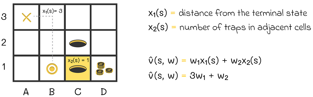
An example of the scalar product used to represent the state value function. The agent’s state is represented by two features. The distance from the agent’s position (B1) to the terminal state (A3) is 3. The adjacent trap cell (C1), with respect to the current agent’s position, is colored in yellow.
According to the described idea, we can add a new feature x₃(s) that will be, for example, the product between x₁(s) and x₂(s). What is the point?
Imagine a situation where the agent is simultaneously very far from the maze exit and surrounded by a large number of traps which means that:
Overall, the agent has a very small chance to successfully escape from the maze in that situation, thus we want the approximated return for this state to be strongly negative.
While x₁(s) and x₂(s) already contain necessary information and can affect the approximated state value, the introduction of x₃(s) = x₁(s) ⋅ x₂(s) adds an additional penalty for this type of situation. Since x₃(s) is a quadratic term, the penalty effect will be tangible. With a good choice of weights w₁, w₂, and w₃, the target state values should significantly be reduced for “bad” agent’s states. At the same time, this effect might not be achievable when only using the original features x₁(s) and x₂(s).
Adding a new term containing information about interaction of features x₁(s) and x₂(s)
Polynomials provide the easiest way to include interaction between features. New features can be derived as a polynomial of the existing features. For instance, let us suppose that there are two features: x₁(s) and x₂(s). We can transform them into the four-dimensional quadratic feature vector x(s):

Quadratic polynomial feature vector. Image adapted by the author. Source: Reinforcement Learning. An Introduction. Second Edition | Richard S. Sutton and Andrew G. Barto
In the example we saw in the previous section, we were using this type of transformation except for the first constant vector component (1). In some cases, it is worth using polynomials of higher degrees. But since the total number of vector components grows exponentially with every next degree, it is usually preferred to choose only a subset of features to reduce optimization computations.

Polynomial feature vector of degree 4. Several components of this vector were omitted. Image adapted by the author. Source: Reinforcement Learning. An Introduction. Second Edition | Richard S. Sutton and Andrew G. Barto
2. Fourier basis
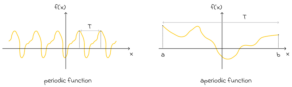
The Fourier series is a beautiful mathematical result that states a periodic function can be approximated as a weighted sum of sine and cosine functions that evenly divide the period T.
Fourier series formula. Image adapted by the author. Source: Fourier series | Wikipedia
To use it effectively in our analysis, we need to go through a pair of important mathematical tricks:
Imagine an aperiodic function defined on an interval [a, b]. Can we still approximate it with the Fourier series? The answer is yes! All we have to do is use the same formula with the period T equal to the length of that interval, b — a.
2. Removing sine terms
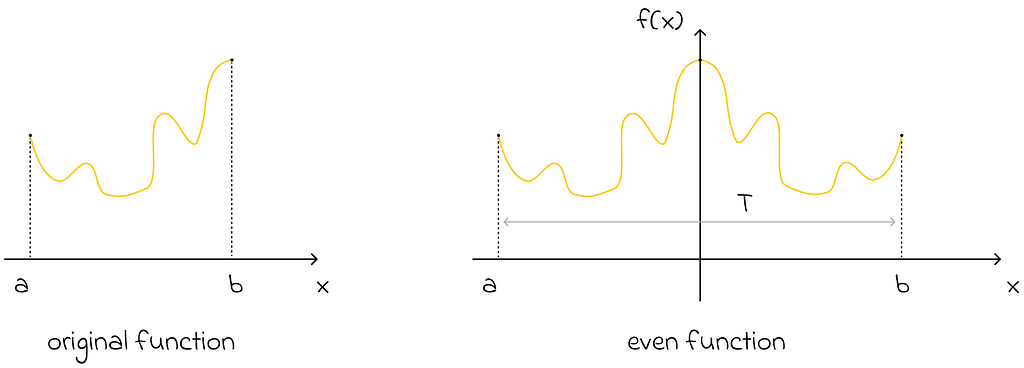
Another important statement, which is not difficult to prove, is that if a function is even, then its Fourier representation contains only cosines (sine terms are equal to 0). Keeping this fact in mind, we can set the period T to be equal to twice the interval length of interest. Then we can perceive the function as being even relative to the middle of its double interval. As a consequence, its Fourier representation will contain only cosines!
The original function can be reflected symmetrically with respect to itself to make it even
Having considered a pair of important mathematical properties, let us now assume that our features are defined on an interval [0, 1] (if not, they can always be normalized). Given that, we set the period T = 2. As a result, the one-dimensional order Fourier basis consists of n + 1 features (n is the maximal frequency term in the Fourier series formula):

One-dimensional Fourier basis
For instance, this is how the one-dimensional Fourier basis looks if n = 5:

Example of one-dimensional Fourier basis (n = 4)
High-dimensional basis
Let us now understand how a high-dimensional basis can be constructed. For simplicity, we will take a vector s consisting of only two components s₁, s₂ each belonging to the interval [0, 1]:
n = 0
This is a trivial case where feature values si are multiplied by 0. As a result, the whole argument of the cosine function is 0. Since the cosine of 0 is equal to 1, the resulting basis is:

Fourier basis example (n = 0)
n = 1
For n = 1, we can take any pairwise combinations of s₁ and s₂ with coefficients -1, 0 and 1, as shown in the image below:
Fourier basis example (n = 1)
For simplicity, the example contains only 4 features. However, in reality, more features can be produced. If there were more than two features, then we could also include new linear terms for other features in the resulting combinations.
n = 2
With n = 2, the principle is the same as in the previous case except for the fact that now the possible coefficient values are -2, -1, 0, 1 and 2.
Fourier basis example (n = 2)
The pattern must be clear now: to construct the Fourier basis for a given value of n, we are allowed to use cosines of any linear combinations of features sᵢ with coefficients whose absolute values are less than or equal to n.
It is easy to see that the number of features grows exponentially with the rise of n. That is why, in a lot of cases, it is necessary to optimally preselect features, to reduce required computations.
State aggregation is a useful technique used to decrease the training complexity. It consists of identifying and grouping similar states together. This way:
This technique can be useful in cases when there are a lot of subsets of similar states. If one clusters them into groups, then the total number of states becomes fewer, thus accelerating the learning process and reducing memory requirements. The flip side of aggregation is less accurate function values used to represent every individual state.
Another possible heuristic for state aggregation consists of mapping every state group to a subset of components of the weight vector w. Different state groups must always be associated with different non-intersecting components of w.
Whenever a gradient is calculated with respect to a given group, only components of the vector w associated with that group are updated. The values of other components do not change.
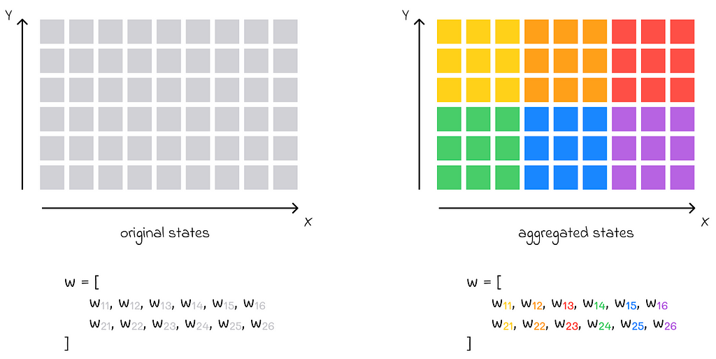
State aggregation example. The original state space on the left consists of a large number of (x, y) coordinate pairs (represented by small gray squares). The aggregated states are shown on the right and highlighted in different colors. Every aggregated state is a group of 3 ⋅ 3 = 9 adjacent states from the diagram on the left. The original weight vector, consisting of 12 components, is now divided into 6 parts, with each part consisting of 2 vector components that correspond to each aggregated state.
We will look at two popular ways of implementing state aggregation in reinforcement learning.
3.1 Coarse coding
Coarse coding consists of representing the whole state space as a set of regions. Every region corresponds to a single binary feature. Every state feature value is determined by the way the state vector is located with respect to a corresponding region:
In addition, regions can overlap between them, meaning that a single state can simultaneously belong to multiple regions. To better illustrate the concept, let us look at the example below.
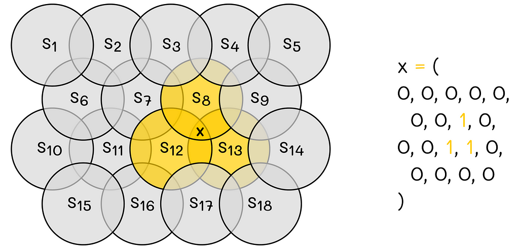
Coarse coding example. Image adapted by the author. Source: Reinforcement Learning. An Introduction. Second Edition | Richard S. Sutton and Andrew G. Barto
In this example, the 2D-space is encoded by 18 circles. The state X belongs to regions 8, 12 and 13. This way, the resulting binary feature vector consists of 18 values where 8-th, 12-th and 13-th components take values of 1, and others take 0.
3.2. Tile coding
Tile coding is similar to coarse coding. In this approach, a geometric object called a tile is chosen and divided into equal subtiles. The tile should cover the whole space. The initial tile is then copied n times, and every copy is positioned in the space with a non-zero offset with respect to the initial tile. The offset size cannot exceed a single subtile size.
This way, if we layer all n tiles together, we will be able to distinguish a large set of small disjoint regions. Every such region will correspond to a binary value in the feature vector depending on how a state is located. To make things simpler, let us proceed to an example.
Let us imagine a 2D-space that is covered by the initial (blue) tile. The tile is divided into 4 ⋅ 4 = 16 equal squares. After that, two other tiles (red and green) of the same shape and structure are created with their respective offsets. As a result, there are 4 ⋅ 4 ⋅ 3 = 48 disjoint regions in total.
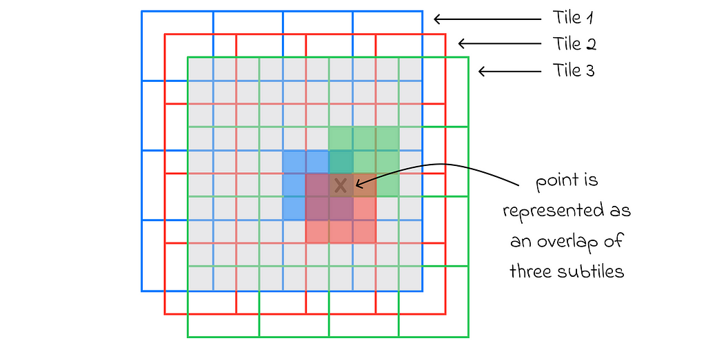
Tile coding example. Image adapted by the author. Source: Reinforcement Learning. An Introduction. Second Edition | Richard S. Sutton and Andrew G. Barto
For any state, its feature vector consists of 48 binary components corresponding to every subtile. To encode the state, for every tile (3 in our case: blue, red, green), one of its subtiles containing the state is chosen. The feature vector component corresponding to the chosen subtile is marked as 1. All unmarked vector values are 0.
Radial basis functions (RBFs) extend the idea of coarse and tile coding, making it possible for feature vector components to take continuous values. This aspect allows for more information about the state to be reflected than just using simple binary values.
A typical RBF basis has a Gaussian form:
Gaussian form of RBF. Image adapted by the author. Source: Reinforcement Learning. An Introduction. Second Edition | Richard S. Sutton and Andrew G. Barto
In this formula,
Example of a one-dimensional RBF basis with a Euclidean distance metric. Source: Reinforcement Learning. An Introduction. Second Edition | Richard S. Sutton and Andrew G. Barto
Another possible option is to describe feature vectors as distances from the state to all protopoints, as shown in the diagram below.
Example of a two-dimensional RBF basis. The feature vector for the given state contains distances to all 9 protopoints.
In this example, there is a two-dimensional coordinate system in the range [0, 1] with 9 protopoints (colored in gray). For any given position of the state vector, the distance between it and all pivot points is calculated. Computed distances form a final feature vector.
*Nonparametric function approximation
Starting from part 7, we have been only discussing parametric methods for value function approximation. In this approach, an algorithm has a set of parameters which it tries to adjust during training in a way that minimizes a loss function value. During inference, the input of a state is run through the latest algorithm’s parameters to evaluate the approximated function value.
Parametric methods’ workflow
Memory-based function approximation
On the other hand, there are memory-based approximation methods. They only have a set of training examples stored in memory that they use during the evaluation of a new state. In contrast to parametric methods, they do not update any parameters. During inference, a subset of training examples is retrieved and used to evaluate a state value.
To illustrate this concept, let us take the example of the linear regression algorithm which uses a linear combination of features to predict values. If there is a quadratic correlation of the predicted variable in relation to the features used, then linear regression will not be able to capture it and, as a result, will perform poorly.
One of the ways to improve the performance of memory-based methods is to increase the number of training examples. During inference, for a given state, it increases the chance that there will be more similar states in the training dataset. This way, the targets of similar training states can be efficiently used to better approximate the desired state value.
Kernel-based function approximation
In addition to memory-based methods, if there are multiple similar states used to evaluate the target of another state, then their individual impact on the final prediction can be weighted depending on how similar they are to the target state. The function used to assign weights to training examples is called a kernel function, or simply a kernel. Kernels can be learned during gradient or semi-gradient methods.
Kernel-based function approximation. The closest states to the query state are highlighted in yellow (in contrast to other gray states). The kernel function takes features of the closest states as input and outputs coefficients kᵢ, representing how much importance each chosen state has with respect to the final prediction. These coefficients are multiplied by the targets of the chosen states and passed to the aggregation function that outputs the final value.
The k-nearest neighbors (kNN) algorithm is a famous example of a nonparametric method. Despite the simplicity, its naive implementation is far from ideal because kNN performs a linear search of the whole dataset to find the closest states during inference. As a consequence, this approach becomes computationally problematic when the dataset size is very large.
kNN algorithm in Euclidean space. The closest state is the one that has the lowest Euclidean distance to the query state.
For that reason, there exist optimization techniques used to accelerate the search. In fact, there is a whole field in machine learning called similarity search.
Similarity Search
Conclusion
Having understood how linear methods work in the previous part, it was essential to dive deeper to gain a complete perspective of how linear algorithms can be improved. As in classical machine learning, feature engineering plays a crucial role in enhancing an algorithm’s performance. Even the most powerful algorithm cannot be efficient without proper feature engineering.
As a result, we have looked at very simplified examples where we dealt with at most dozens of features. In reality, the number of features derived from a state can be much larger. To efficiently solve a reinforcement learning problem in real life, a basis consisting of thousands of features can be used!
Finally, the introduction to nonparametric function approximation methods served as a robust approach for solving the original problem while not limiting the solution to a predefined class of functions.
Resources
All images unless otherwise noted are by the author.

Reinforcement Learning, Part 8: Feature State Construction was originally published in Towards Data Science on Medium, where people are continuing the conversation by highlighting and responding to this story.
Reinforcement learning is a domain in machine learning that introduces the concept of an agent learning optimal strategies in complex environments. The agent learns from its actions, which result in rewards, based on the environment’s state. Reinforcement learning is a challenging topic and differs significantly from other areas of machine learning.
What is remarkable about reinforcement learning is that the same algorithms can be used to enable the agent adapt to completely different, unknown, and complex conditions.
About this article
In part 7, we introduced value-function approximation algorithms which scale standard tabular methods. Apart from that, we particularly focused on a very important case when the approximated value function is linear. As we found out, the linearity provides guaranteed convergence either to the global optimum or to the TD fixed point (in semi-gradient methods).
The problem is that sometimes we might want to use a more complex approximation value function, rather than just a simple scalar product, without leaving the linear optimization space. The motivation behind using complex approximation functions is the fact that they fail to account for any information of interaction between features. Since the true state values might have a very sophisticated functional dependency on the input features, their simple linear form might not be enough for good approximation.
In this article, we will understand how to efficiently inject more valuable information about state features into the objective without leaving the linear optimization space.
Note. To fully understand the concepts included in this article, it is highly recommended to be familiar with concepts discussed in previous articles.
Reinforcement Learning
Idea
Problem
Imagine a state vector containing features related to the state:
As we know, this vector is multiplied by the weight vector w, which we would like to find:
Due to the linearity constraint, we cannot simply include other terms containing interactions between coefficients of w. For instance, adding the term w₁w₂ makes the optimization problem quadratic:
For semi-gradient methods, we do not know how to optimize such objectives.
Solution
If you remember the previous part, you know that we can include any information about the state into the feature vector x(s). So if we want to add interaction between features into the objective, why not simply derive new features containing that information?
Let us return to the maze example in the previous article. As a reminder, we originally had two features representing the agent’s state as shown in the image below:
An example of the scalar product used to represent the state value function. The agent’s state is represented by two features. The distance from the agent’s position (B1) to the terminal state (A3) is 3. The adjacent trap cell (C1), with respect to the current agent’s position, is colored in yellow.
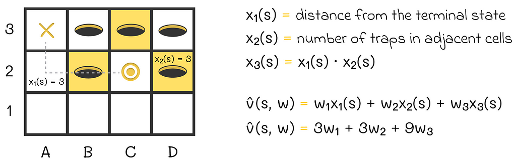
According to the described idea, we can add a new feature x₃(s) that will be, for example, the product between x₁(s) and x₂(s). What is the point?
Imagine a situation where the agent is simultaneously very far from the maze exit and surrounded by a large number of traps which means that:
- x₁(s) >> 1
- x₂(s) >> 1
Overall, the agent has a very small chance to successfully escape from the maze in that situation, thus we want the approximated return for this state to be strongly negative.
While x₁(s) and x₂(s) already contain necessary information and can affect the approximated state value, the introduction of x₃(s) = x₁(s) ⋅ x₂(s) adds an additional penalty for this type of situation. Since x₃(s) is a quadratic term, the penalty effect will be tangible. With a good choice of weights w₁, w₂, and w₃, the target state values should significantly be reduced for “bad” agent’s states. At the same time, this effect might not be achievable when only using the original features x₁(s) and x₂(s).
Adding a new term containing information about interaction of features x₁(s) and x₂(s)
We have just seen an example of a quadratic feature basis. In fact, there exists many basis families that will be explained in the next sections.
1. PolynomialsPolynomials provide the easiest way to include interaction between features. New features can be derived as a polynomial of the existing features. For instance, let us suppose that there are two features: x₁(s) and x₂(s). We can transform them into the four-dimensional quadratic feature vector x(s):
Quadratic polynomial feature vector. Image adapted by the author. Source: Reinforcement Learning. An Introduction. Second Edition | Richard S. Sutton and Andrew G. Barto
In the example we saw in the previous section, we were using this type of transformation except for the first constant vector component (1). In some cases, it is worth using polynomials of higher degrees. But since the total number of vector components grows exponentially with every next degree, it is usually preferred to choose only a subset of features to reduce optimization computations.
Polynomial feature vector of degree 4. Several components of this vector were omitted. Image adapted by the author. Source: Reinforcement Learning. An Introduction. Second Edition | Richard S. Sutton and Andrew G. Barto
2. Fourier basis
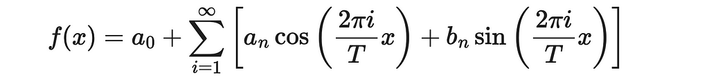
The Fourier series is a beautiful mathematical result that states a periodic function can be approximated as a weighted sum of sine and cosine functions that evenly divide the period T.
Fourier series formula. Image adapted by the author. Source: Fourier series | Wikipedia
To use it effectively in our analysis, we need to go through a pair of important mathematical tricks:
- Omitting the periodicity constraint
Imagine an aperiodic function defined on an interval [a, b]. Can we still approximate it with the Fourier series? The answer is yes! All we have to do is use the same formula with the period T equal to the length of that interval, b — a.
2. Removing sine terms
Another important statement, which is not difficult to prove, is that if a function is even, then its Fourier representation contains only cosines (sine terms are equal to 0). Keeping this fact in mind, we can set the period T to be equal to twice the interval length of interest. Then we can perceive the function as being even relative to the middle of its double interval. As a consequence, its Fourier representation will contain only cosines!
The original function can be reflected symmetrically with respect to itself to make it even
In general, using only cosines simplifies the analysis and reduces computations.
One-dimensional basisHaving considered a pair of important mathematical properties, let us now assume that our features are defined on an interval [0, 1] (if not, they can always be normalized). Given that, we set the period T = 2. As a result, the one-dimensional order Fourier basis consists of n + 1 features (n is the maximal frequency term in the Fourier series formula):
One-dimensional Fourier basis
For instance, this is how the one-dimensional Fourier basis looks if n = 5:
Example of one-dimensional Fourier basis (n = 4)
High-dimensional basis
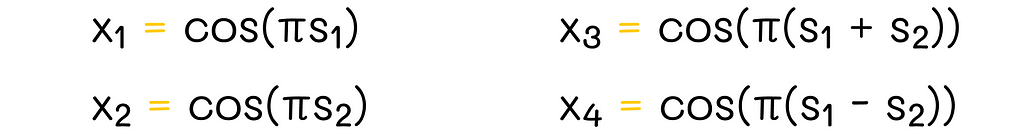
Let us now understand how a high-dimensional basis can be constructed. For simplicity, we will take a vector s consisting of only two components s₁, s₂ each belonging to the interval [0, 1]:
n = 0
This is a trivial case where feature values si are multiplied by 0. As a result, the whole argument of the cosine function is 0. Since the cosine of 0 is equal to 1, the resulting basis is:
Fourier basis example (n = 0)
n = 1
For n = 1, we can take any pairwise combinations of s₁ and s₂ with coefficients -1, 0 and 1, as shown in the image below:
Fourier basis example (n = 1)
For simplicity, the example contains only 4 features. However, in reality, more features can be produced. If there were more than two features, then we could also include new linear terms for other features in the resulting combinations.
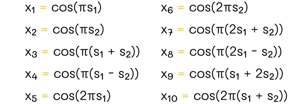
n = 2
With n = 2, the principle is the same as in the previous case except for the fact that now the possible coefficient values are -2, -1, 0, 1 and 2.
Fourier basis example (n = 2)
The pattern must be clear now: to construct the Fourier basis for a given value of n, we are allowed to use cosines of any linear combinations of features sᵢ with coefficients whose absolute values are less than or equal to n.
It is easy to see that the number of features grows exponentially with the rise of n. That is why, in a lot of cases, it is necessary to optimally preselect features, to reduce required computations.
In practice, Fourier basis is usually more effective than the polynomial basis.
3. State aggregationState aggregation is a useful technique used to decrease the training complexity. It consists of identifying and grouping similar states together. This way:
- Grouped states share the same state value.
- Whenever an update affects a single state, it also affects all states of that group.
This technique can be useful in cases when there are a lot of subsets of similar states. If one clusters them into groups, then the total number of states becomes fewer, thus accelerating the learning process and reducing memory requirements. The flip side of aggregation is less accurate function values used to represent every individual state.
Another possible heuristic for state aggregation consists of mapping every state group to a subset of components of the weight vector w. Different state groups must always be associated with different non-intersecting components of w.
Whenever a gradient is calculated with respect to a given group, only components of the vector w associated with that group are updated. The values of other components do not change.
State aggregation example. The original state space on the left consists of a large number of (x, y) coordinate pairs (represented by small gray squares). The aggregated states are shown on the right and highlighted in different colors. Every aggregated state is a group of 3 ⋅ 3 = 9 adjacent states from the diagram on the left. The original weight vector, consisting of 12 components, is now divided into 6 parts, with each part consisting of 2 vector components that correspond to each aggregated state.
We will look at two popular ways of implementing state aggregation in reinforcement learning.
3.1 Coarse coding
Coarse coding consists of representing the whole state space as a set of regions. Every region corresponds to a single binary feature. Every state feature value is determined by the way the state vector is located with respect to a corresponding region:
- 0: the state is outside the region;
- 1: the state is inside the region.
In addition, regions can overlap between them, meaning that a single state can simultaneously belong to multiple regions. To better illustrate the concept, let us look at the example below.
Coarse coding example. Image adapted by the author. Source: Reinforcement Learning. An Introduction. Second Edition | Richard S. Sutton and Andrew G. Barto
In this example, the 2D-space is encoded by 18 circles. The state X belongs to regions 8, 12 and 13. This way, the resulting binary feature vector consists of 18 values where 8-th, 12-th and 13-th components take values of 1, and others take 0.
3.2. Tile coding
Tile coding is similar to coarse coding. In this approach, a geometric object called a tile is chosen and divided into equal subtiles. The tile should cover the whole space. The initial tile is then copied n times, and every copy is positioned in the space with a non-zero offset with respect to the initial tile. The offset size cannot exceed a single subtile size.
This way, if we layer all n tiles together, we will be able to distinguish a large set of small disjoint regions. Every such region will correspond to a binary value in the feature vector depending on how a state is located. To make things simpler, let us proceed to an example.
Let us imagine a 2D-space that is covered by the initial (blue) tile. The tile is divided into 4 ⋅ 4 = 16 equal squares. After that, two other tiles (red and green) of the same shape and structure are created with their respective offsets. As a result, there are 4 ⋅ 4 ⋅ 3 = 48 disjoint regions in total.
Tile coding example. Image adapted by the author. Source: Reinforcement Learning. An Introduction. Second Edition | Richard S. Sutton and Andrew G. Barto
For any state, its feature vector consists of 48 binary components corresponding to every subtile. To encode the state, for every tile (3 in our case: blue, red, green), one of its subtiles containing the state is chosen. The feature vector component corresponding to the chosen subtile is marked as 1. All unmarked vector values are 0.
Since exactly one subtile for a given tile is chosen every time, it is guaranteed that any state is always represented by a binary vector containing exactly n values of 1. This property is useful in some algorithms, making their adjustment of learning rate more stable.
4. Radial basis functionsRadial basis functions (RBFs) extend the idea of coarse and tile coding, making it possible for feature vector components to take continuous values. This aspect allows for more information about the state to be reflected than just using simple binary values.
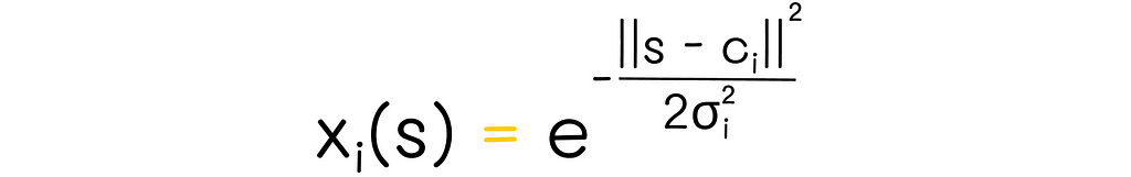
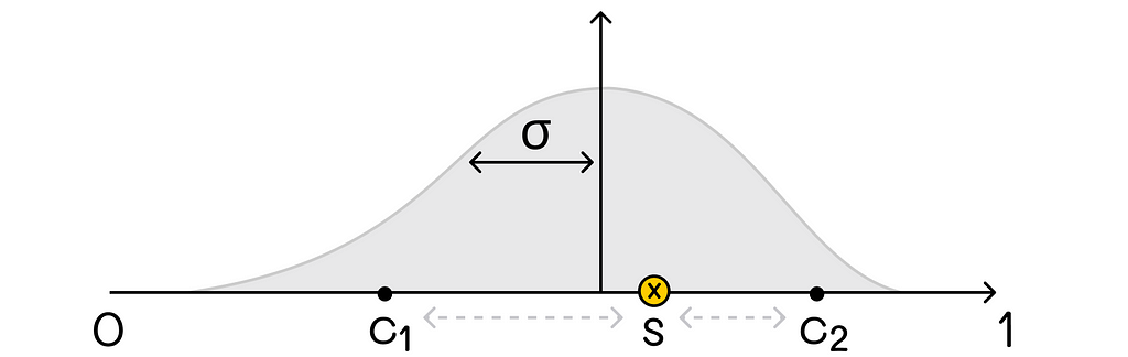
A typical RBF basis has a Gaussian form:
Gaussian form of RBF. Image adapted by the author. Source: Reinforcement Learning. An Introduction. Second Edition | Richard S. Sutton and Andrew G. Barto
In this formula,
- s: state;
- cᵢ: a feature protopoint which is usually chosen as a feature’s center;
- || s — cᵢ ||: the distance between the state s and a protopoint ci. This distance metric can be customarily chosen (i.e. Euclidean distance).
- σ: feature’s width which is a measure that describes the relative range of feature values. Standard deviation is one of the examples of feature width.
Example of a one-dimensional RBF basis with a Euclidean distance metric. Source: Reinforcement Learning. An Introduction. Second Edition | Richard S. Sutton and Andrew G. Barto
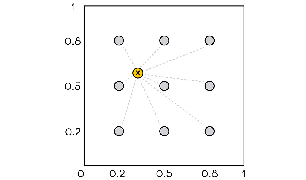
Another possible option is to describe feature vectors as distances from the state to all protopoints, as shown in the diagram below.
Example of a two-dimensional RBF basis. The feature vector for the given state contains distances to all 9 protopoints.
In this example, there is a two-dimensional coordinate system in the range [0, 1] with 9 protopoints (colored in gray). For any given position of the state vector, the distance between it and all pivot points is calculated. Computed distances form a final feature vector.
*Nonparametric function approximation
Though this section is not related to state feature construction, understanding the idea of nonparametric methods opens up doors to new types of algorithms. A combination with appropriate feature engineering techniques discussed above can improve performance in some circumstances.
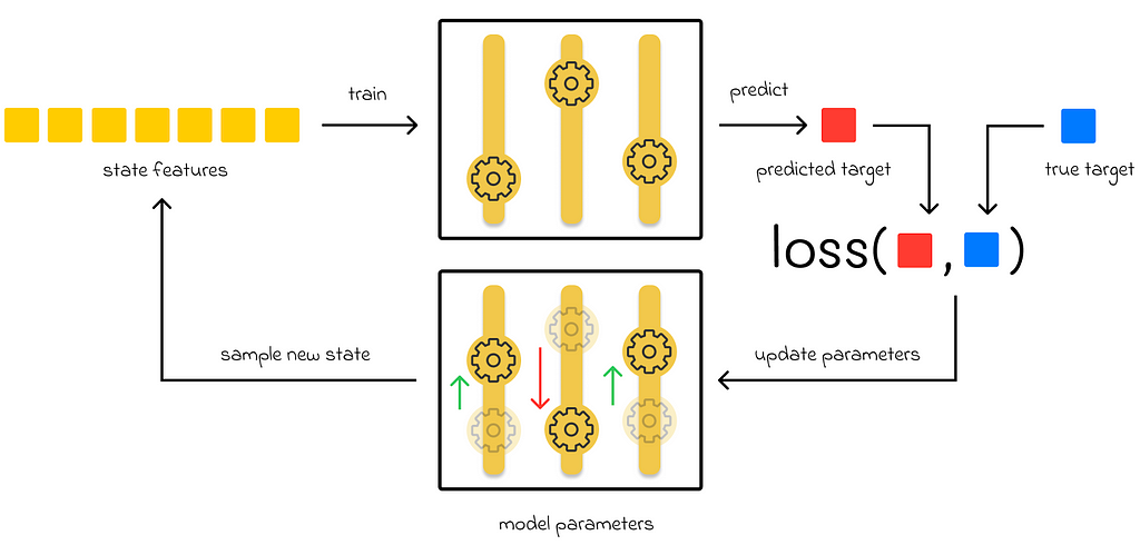
Starting from part 7, we have been only discussing parametric methods for value function approximation. In this approach, an algorithm has a set of parameters which it tries to adjust during training in a way that minimizes a loss function value. During inference, the input of a state is run through the latest algorithm’s parameters to evaluate the approximated function value.
Parametric methods’ workflow
Memory-based function approximation
On the other hand, there are memory-based approximation methods. They only have a set of training examples stored in memory that they use during the evaluation of a new state. In contrast to parametric methods, they do not update any parameters. During inference, a subset of training examples is retrieved and used to evaluate a state value.
Sometimes the term “lazy learning” is used to describe nonparametric methods because they do not have any training phase and make computations only when evaluation is needed during inference.
The advantage of memory-based methods is that their approximation method is not limited a given class of functions, which is the case for parametric methods.
To illustrate this concept, let us take the example of the linear regression algorithm which uses a linear combination of features to predict values. If there is a quadratic correlation of the predicted variable in relation to the features used, then linear regression will not be able to capture it and, as a result, will perform poorly.
One of the ways to improve the performance of memory-based methods is to increase the number of training examples. During inference, for a given state, it increases the chance that there will be more similar states in the training dataset. This way, the targets of similar training states can be efficiently used to better approximate the desired state value.
Kernel-based function approximation
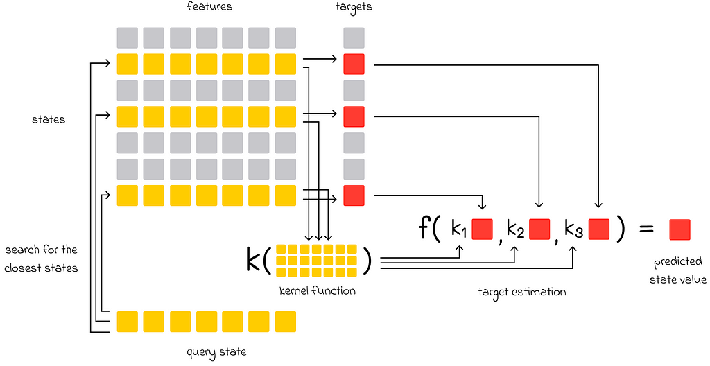
In addition to memory-based methods, if there are multiple similar states used to evaluate the target of another state, then their individual impact on the final prediction can be weighted depending on how similar they are to the target state. The function used to assign weights to training examples is called a kernel function, or simply a kernel. Kernels can be learned during gradient or semi-gradient methods.
Kernel-based function approximation. The closest states to the query state are highlighted in yellow (in contrast to other gray states). The kernel function takes features of the closest states as input and outputs coefficients kᵢ, representing how much importance each chosen state has with respect to the final prediction. These coefficients are multiplied by the targets of the chosen states and passed to the aggregation function that outputs the final value.
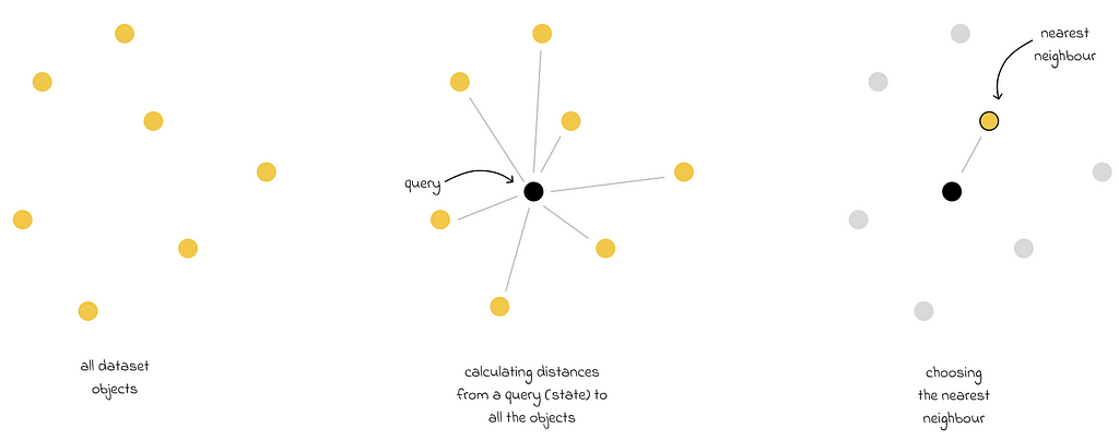
The k-nearest neighbors (kNN) algorithm is a famous example of a nonparametric method. Despite the simplicity, its naive implementation is far from ideal because kNN performs a linear search of the whole dataset to find the closest states during inference. As a consequence, this approach becomes computationally problematic when the dataset size is very large.
kNN algorithm in Euclidean space. The closest state is the one that has the lowest Euclidean distance to the query state.
For that reason, there exist optimization techniques used to accelerate the search. In fact, there is a whole field in machine learning called similarity search.
If you are interested in exploring the most popular algorithms to scale search for large datasets, then I recommend checking out the “Similarity Search” series.
Similarity Search
Conclusion
Having understood how linear methods work in the previous part, it was essential to dive deeper to gain a complete perspective of how linear algorithms can be improved. As in classical machine learning, feature engineering plays a crucial role in enhancing an algorithm’s performance. Even the most powerful algorithm cannot be efficient without proper feature engineering.
As a result, we have looked at very simplified examples where we dealt with at most dozens of features. In reality, the number of features derived from a state can be much larger. To efficiently solve a reinforcement learning problem in real life, a basis consisting of thousands of features can be used!
Finally, the introduction to nonparametric function approximation methods served as a robust approach for solving the original problem while not limiting the solution to a predefined class of functions.
Resources
- Reinforcement Learning. An Introduction. Second Edition | Richard S. Sutton and Andrew G. Barto
- Fourier series | Wikipedia
All images unless otherwise noted are by the author.
Reinforcement Learning, Part 8: Feature State Construction was originally published in Towards Data Science on Medium, where people are continuing the conversation by highlighting and responding to this story.