Why is K-Means the most popular algorithm in Unsupervised Learning? Let’s dive into its math, and build it from scratch.

Image generated by DALL-E
K-means clustering is a staple in machine learning for its straightforward approach to organizing complex data. In this article we’ll explore the core of the algorithm. We will delve into its applications, dissect the math behind it, build it from scratch, and discuss its relevance in the fast-evolving field of data science.
Index
· 1: Understanding the Basics
∘ 1.1: What is K-Means Clustering?
∘ 1.2: How Does K-Means Work?
· 2: Implementing K-Means
∘ 2.1: The Mathematics Behind K-Means
∘ 2.2: Choosing the Optimal Number of Clusters
· 3: K-Means in Practice
∘ 3.1 K-Means From Scratch in Python
∘ 3.2 Implementing K-Means with Scikit-Learn
· 4: Advantages and Challenges
∘ 4.1 Benefits of Using K-Means
∘ 4.2 Overcoming K-Means Limitations
· 5: Beyond Basic K-Means
∘ 5.1 Variants of K-Means
· 6: Conclusion
· Bibliography
1: Understanding the Basics
1.1: What is K-Means Clustering?

Image generated by DALL-E
Imagine you’re at a farmer’s market with a bunch of fruits and veggies that you need to sort out. You want to organize them so all the apples, oranges, and carrots are hanging out with their kind. This task is a lot like what K-Means Clustering does in data science.
So, what’s K-Means Clustering? It’s a technique used to naturally group data. Think of it as a way to sort unlabeled data into different groups or clusters. Each cluster is a bunch of data points that are more alike to each other than to those in other groups. The “K” in K-Means? It represents the number of groups you think there should be.
1.2: How Does K-Means Work?
Now, keep in mind the farmer’s market example, and let’s try to dive deep a bit more into K-means mechanisms.
Think of K-Means as setting up the initial fruit stands (centroids) in our market. It randomly picks a few spots (data points) to place these stands. The number of stands you decide to set up is the “K” in K-Means, and this number depends on how many different types of produce (groups) you think you have.
Now, K-Means takes each fruit and veggie (data point) and figures out which stand (centroid) it belongs to based on how close it is. It’s like each apple, orange, or carrot choosing the closest stand to hang out at, forming little groups around them.
After all the produce has found a stand, K-Means checks if the stands are in the best spots. It does this by finding a new spot for each stand based on the average position of all the produce grouped around them. It’s similar to moving the stands to the exact middle of each produce group to make sure they’re truly at the heart of the action.
This process of sorting produce and adjusting stands keeps going. Fruits and veggies might move to a different stand if they find one closer, and the stands might shift positions to better represent their groups. This cycle continues until the stands and their produce groups don’t change much anymore. That’s when K-Means knows the market is perfectly organized, and every piece of produce is of its kind.

Image generated by DALL-E
What you end up with are nicely organized stands (clusters) with fruits and veggies grouped around them. Each stand represents a type of produce, showing you how your market (data) can be divided into distinct sections (categories) based on similarities.
2: Implementing K-Means
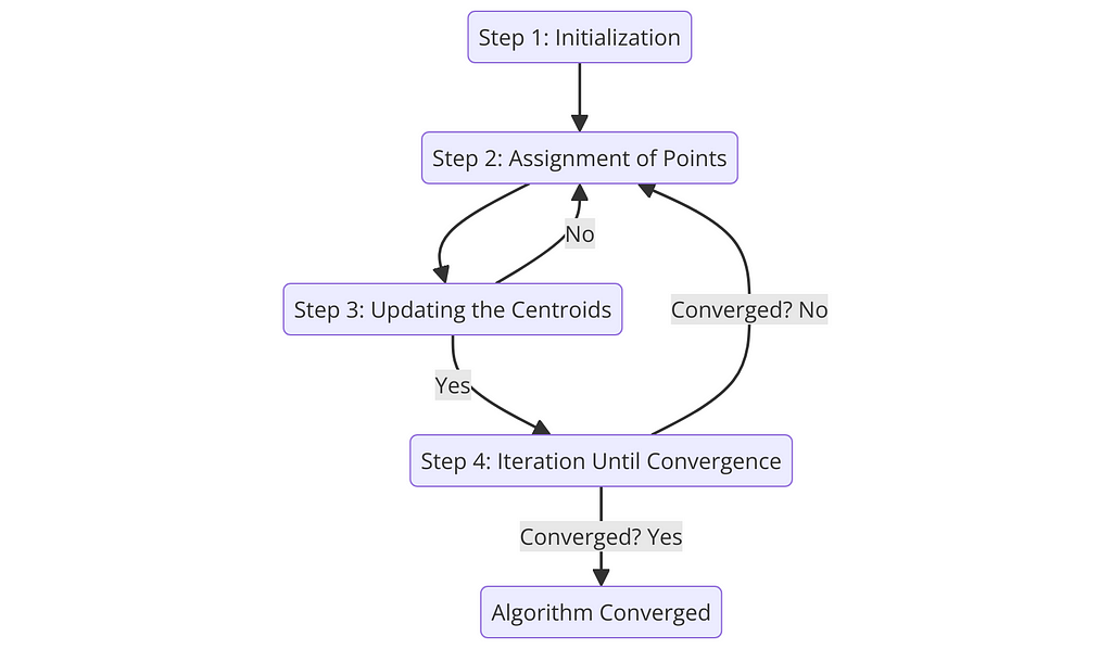
K-Means Step Chart — Image by Author
2.1: The Mathematics Behind K-Means
Let’s put on our math hats for a moment and peek into the engine room of the K-Means algorithm to see what makes it tick. K-Means is all about finding the sweet spot:
Here’s how the math plays out:
Step 1: Initialization
Initially, K-Means needs to decide where to start, choosing k initial centroids (μ1,μ2,…,μk) from the dataset. This can be done randomly or more strategically with methods like K-Means++, which we will cover later.
While no specific formula is used here, the choice of initial centroids can significantly affect the outcome. But don’t worry, because, in the next section, we will guide you through the best tips to choose the optimal k.
Step 2: Assignment of Points to Closest Centroid
NeXT, each data point x is assigned to the nearest centroid, forming k clusters, where the “nearest” centroid is determined by the minimum distance between the point and all centroids.
Here, the distance d between a point x and a centroid μi is typically calculated using the Euclidean distance:
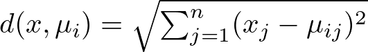
Euclidean distance formula — Image by Author
where xj and μij are the j-th dimensions of point x and centroid μi, respectively. Now, while Euclidean distance is the most popular choice for K-Means, you could explore its application with more distances. However, keep in mind that Euclidean distance is usually the suggested choice for optimal performance, whereas other variances of the algorithm are more flexible to different distance methods. Look at the subsection 2.1 of my previous article about K-Nearest Neighbors to know more about distance methods:
The Math Behind K-Nearest Neighbors
Keeping the Euclidean distance in mind, let’s see how the algorithm assigns a point x to the cluster Ci:

Assignment of x to cluster condition — Image by Author
Here’s what it means:
The condition d(x,μi) ≤ d(x,μj) ∀ j, 1≤j≤k specifies that a point x is assigned to the cluster Ci if and only if the distance from x to the centroid μi of Ci is less than or equal to its distance from x to the centroids μj of all other clusters Cj, for every j from 1 to k.
In simpler terms, the formula says:
This step ensures that each point is assigned to the cluster with the nearest centroid, minimizing within-cluster distances and making the clusters as tight and homogenous as possible.
Step 3: Updating the Centroids
After all points have been assigned to clusters, the positions of the centroids are recalculated to be at the center of their respective clusters.
The new position μi′ of centroid μi is calculated as the mean of all points assigned to cluster Ci:
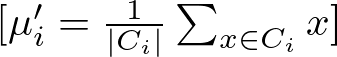
Centroid position’s update formula — Image by Author
where ∣Ci∣ is the number of points in cluster Ci, and the summation aggregates the positions of all points in the cluster.
Step 4: Iteration Until Convergence
The assignment and update steps (Steps 2 and 3) are repeated until the centroids no longer change significantly, indicating that the algorithm has converged.
Here, convergence is typically assessed by measuring the change in centroid positions between iterations. If the change falls below a predetermined threshold, the algorithm stops.
In the context of the K-Means algorithm, there isn’t a single, universally defined formula for convergence that applies in all cases. Instead, convergence is determined based on the algorithm's behavior over successive iterations, specifically whether the centroids of the clusters stop changing significantly.
However, a common way to assess convergence is by looking at the change in the within-cluster sum of squares (WCSS) or the positions of the centroids between iterations. Here, we set a threshold for changes in the centroid positions or the WCSS. If the change falls below this threshold from one iteration to the next, the algorithm can be considered to have converged. This can be expressed as:
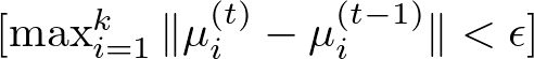
Convergence formula — Image by Author
where:
Deciding on the right number of clusters, k, in K-Means clustering is more art than science. It’s like Goldilocks trying to find the bed that’s just right, with not too many clusters to overcomplicate things, and not too few to oversimplify. Here’s how you can find that sweet spot:
The Elbow Method
One popular technique is the Elbow Method. It involves running K-Means several times, each time with a different number of clusters, and then plotting the Within-Cluster Sum of Squares (WCSS) against the number of clusters. WCSS measures how tight your clusters are, with lower values indicating that points are closer to their respective centroids.
The formula for calculating WCSS is :

Within-Cluster Sum of Squares Formula — Image by Author
Here’s a breakdown of this formula:
The WCSS is essentially a sum of these squared distances for all points in each cluster, aggregated across all k clusters. A lower WCSS value indicates that points are on average closer to their cluster centroids, suggesting tighter and possibly more meaningful clusters.
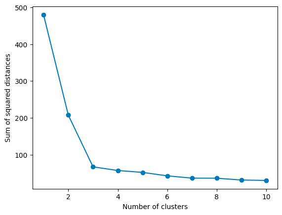
The sum of Squared Distances by K Plot — Image by Author
As you increase k, WCSS decreases because the points are closer to centroids. However, there’s a point where adding more clusters doesn’t give you much bang for your buck. This point, where the rate of decrease sharply changes, looks like an elbow on the graph. In the graph above, the elbow point is 3, as the rate of decrease slows down significantly afterward. That’s your Goldilocks k:
The Silhouette Method
Another approach is the Silhouette Method, which evaluates how similar an object is to its cluster compared to other clusters. The silhouette score ranges from -1 to 1, where a high value indicates that the object is well-matched to its cluster and poorly matched to neighboring clusters.
The formula for calculating the Silhouette Score for a single data point is:
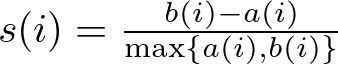
Silhouette Score Formula — Image by Author
Then, we take the average silhouette score for the dataset, which is calculated by averaging the silhouette scores of all points. In mathematical terms:

Average Silhouette Score Formula — Image by Author
where N is the total number of points in the dataset.
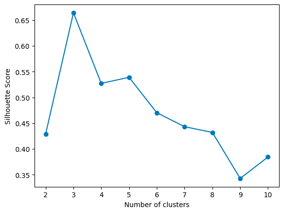
Silhouette Score by K — Image by Author
For each k, calculate the average silhouette score of all points. The k that gives you the highest average silhouette score is considered the optimal number of clusters. It’s like finding the party where everyone feels they fit in best. In the graph above, the highest score is given by 3 clusters.
K-Means++
Means++ is an algorithm for choosing the initial values (or “seeds”) for the K-Means clustering algorithm. The standard K-Means algorithm starts with a random selection of centroids, which can sometimes result in poor convergence speed and suboptimal clustering. K-Means++ addresses this by spreading out the initial centroids before proceeding with the standard K-Means optimization iterations.
It begins by randomly selecting the first centroid from the dataset. Then, for each subsequent centroid, K-Means++ chooses data points as new centroids with a probability proportional to their squared distance from the nearest existing centroid. This step increases the chances of selecting centroids that are far away from each other, reducing the likelihood of poor clustering. This process is repeated until all k centroids are chosen.
Lastly, once the initial centroids are selected using the K-Means++ approach, continue with the standard K-Means algorithm to adjust the centroids and assign points to clusters.
In this post, I won’t delve deep into K-Means++ math, but expect it in a new post. In the meantime, you could read the following article for a better understanding:
k-means++: The Advantages of Careful Seeding
3: K-Means in Practice
3.1 K-Means From Scratch in Python
As I like to do in this “Machine Learning From Scratch” series, let’s now recreate a simpler version of the algorithm from scratch. Let’s first look at the whole code:
class KMeans:
def __init__(self, K, max_iters=100, tol=1e-4):
"""
Constructor for KMeans class
Parameters
----------
K : int
Number of clusters
max_iters : int, optional
Maximum number of iterations, by default 100
tol : float, optional
Tolerance to declare convergence, by default 1e-4
"""
self.K = K
self.max_iters = max_iters
self.tol = tol
self.centroids = None
self.labels = None
self.inertia_ = None
def initialize_centroids(self, X):
"""
Initialize centroids
Parameters
----------
X : array-like
Input data
Returns
-------
array-like
Initial centroids
"""
# Simple random initialization, consider k-means++ for improvement
indices = np.random.permutation(X.shape[0])
centroids = X[indices[:self.K]]
return centroids
def compute_centroids(self, X, labels):
"""
Compute centroids
Parameters
----------
X : array-like
Input data
labels : array-like
Cluster labels
Returns
-------
array-like
Updated centroids
"""
centroids = np.zeros((self.K, X.shape[1]))
for k in range(self.K):
if np.any(labels == k):
centroids[k] = np.mean(X[labels == k], axis=0)
else:
centroids[k] = X[np.random.choice(X.shape[0])]
return centroids
def compute_distance(self, X, centroids):
"""
Compute distances between data points and centroids
Parameters
----------
X : array-like
Input data
centroids : array-like
Centroids
Returns
-------
array-like
Distances
"""
distances = np.zeros((X.shape[0], self.K))
for k in range(self.K):
distances[:, k] = np.linalg.norm(X - centroids[k], axis=1) ** 2
return distances
def find_closest_cluster(self, distances):
"""
Find the closest cluster for each data point
Parameters
----------
distances : array-like
Distances
Returns
-------
array-like
Cluster labels
"""
return np.argmin(distances, axis=1)
def fit(self, X):
"""
Fit the model
Parameters
----------
X : array-like
Input data
"""
self.centroids = self.initialize_centroids(X)
for i in range(self.max_iters):
distances = self.compute_distance(X, self.centroids)
self.labels = self.find_closest_cluster(distances)
new_centroids = self.compute_centroids(X, self.labels)
# Compute inertia (sum of squared distances)
inertia = np.sum([distances[i, label] for i, label in enumerate(self.labels)])
# Check for convergence: if the centroids don't change much (within tolerance)
if np.allclose(self.centroids, new_centroids, atol=self.tol) or inertia <= self.tol:
break
self.centroids = new_centroids
self.inertia_ = inertia
def predict(self, X):
"""
Predict the closest cluster for each data point
Parameters
----------
X : array-like
Input data
Returns
-------
array-like
Cluster labels
"""
distances = self.compute_distance(X, self.centroids)
return self.find_closest_cluster(distances)
Let’s break down each part of the class to explain its functionality:
def __init__(self, K, max_iters=100, tol=1e-4):
self.K = K
self.max_iters = max_iters
self.tol = tol
self.centroids = None
self.labels = None
self.inertia_ = None
This method initializes a new instance of the KMeans class.
Here, the parameters are:
We also initialize a few attributes to None:
2. initialize_centroids and compute_centroids Methods:
def initialize_centroids(self, X):
# Simple random initialization, consider k-means++ for improvement
indices = np.random.permutation(X.shape[0])
centroids = X[indices[:self.K]]
return centroids
def compute_centroids(self, X, labels):
centroids = np.zeros((self.K, X.shape[1]))
for k in range(self.K):
if np.any(labels == k):
centroids[k] = np.mean(X[labels == k], axis=0)
else:
centroids[k] = X[np.random.choice(X.shape[0])]
return centroids
First, we initialize the centroids randomly from the data points, by randomly permuting the indices of the input data and selecting the first K as the initial centroids. As we mentioned before, a random selection is one of the possible centroid initializations, you could go ahead and experiment with more techniques to see how this affects the performance of the model.
Then, we compute the new centroids as the mean of the data points assigned to each cluster. Here, if a cluster ends up with no points, a random data point from X is chosen as the new centroid for that cluster.
3. compute_distance and find_closest_clusterMethod:
def compute_distance(self, X, centroids):
distances = np.zeros((X.shape[0], self.K))
for k in range(self.K):
distances[:, k] = np.linalg.norm(X - centroids[k], axis=1) ** 2
return distances
def find_closest_cluster(self, distances):
return np.argmin(distances, axis=1)
We define the method to calculate the squared Euclidean distance between each data point and each centroid, which returns an array where each element contains the squared distances from a data point to all centroids.
Then, we assign each data point to the closest cluster based on the computed distances. The output of the operation consists of an array of labels indicating the closest cluster for each data point.
4. fit and predict Method:
def fit(self, X):
self.centroids = self.initialize_centroids(X)
for i in range(self.max_iters):
distances = self.compute_distance(X, self.centroids)
self.labels = self.find_closest_cluster(distances)
new_centroids = self.compute_centroids(X, self.labels)
# Compute inertia (sum of squared distances)
inertia = np.sum([distances[i, label] for i, label in enumerate(self.labels)])
# Check for convergence: if the centroids don't change much (within tolerance)
if np.allclose(self.centroids, new_centroids, atol=self.tol) or inertia <= self.tol:
break
self.centroids = new_centroids
self.inertia_ = inertia
def predict(self, X):
distances = self.compute_distance(X, self.centroids)
return self.find_closest_cluster(distances)
Now we build the core method of this class: the fit method, which first initializes the centroids, and iterates up to max_iters times, where in each iteration:
Lastly, we predict the closest cluster for each point in a new dataset, using the predict method.
You can find the whole code and a practical implementation in this Jupyter Notebook:
models-from-scratch-python/K-Means/demo.ipynb at main · cristianleoo/models-from-scratch-python
3.2 Implementing K-Means with Scikit-Learn
Ok, now you have a solid understanding of what the algorithm does, and you can recreate the algorithm from scratch. Pretty cool right? Well, you won’t be using that code anytime soon, as our friend Scikit Learn already provides a much more efficient implementation of K-Means, which only takes a few lines of code. Here, we can use variations of K-Means only by specifying a parameter. Let’s look at one implementation of it.
from sklearn.cluster import KMeans
from sklearn.datasets import make_blobs
# Generate a synthetic dataset
X, y_true = make_blobs(n_samples=300, centers=3, cluster_std=0.60, random_state=0)
# Initialize and fit KMeans
kmeans = KMeans(n_clusters=3, max_iter=100, tol=1e-4)
kmeans.fit(X)
# Predict the cluster labels
labels = kmeans.predict(X)
# Print the cluster centers
print("Cluster centers:\n", kmeans.cluster_centers_)
We first import KMeans from scikit-learn, and make_blobs is a function to generate synthetic datasets for clustering. We generate a synthetic dataset with 300 samples, 3 centers (clusters), and a standard deviation of 0.60 for each cluster. The random_state parameter is used to ensure that the results are reproducible.
We initialize the KMeans algorithm with 3 clusters (n_clusters=3), a maximum of 100 iterations (max_iter=100), and a tolerance of 1e-4 (tol=1e-4). The tolerance is the threshold to declare convergence — if the change in the within-cluster sum of squares (inertia) is less than this value, the algorithm will stop.
We fit the KMeans algorithm to our data using the fit method. This is where the actual clustering happens. We predict the cluster labels for our data using the predict method. This assigns each data point to the nearest cluster.
sklearn.cluster.KMeans
4: Advantages and Challenges
4.1 Benefits of Using K-Means
At this point, you probably have an idea of why K-Means is so popular, but let’s make sure you know when to consider K-Means for your data science journey:
Simplicity and Ease of Implementation
First off, K-Means is straightforward. It doesn’t ask for much, just the data and the number of clusters k you’re aiming for. This simplicity makes it super approachable, even for beginners in the data science field.
Efficiency at Scale
K-Means is pretty efficient, especially with large datasets. It’s got a way of cutting through data to find patterns without needing a supercomputer to do its thing. This efficiency makes it a practical choice for real-world applications where time and resources are of the essence.
Good for Pre-Processing and Simplification
The algorithm can also be a great pre-processing step. By clustering your data first, you can simplify complex problems, reduce dimensionality, or even improve the performance of other algorithms that you might run afterward.
Discovering Patterns and Insights
It can help uncover hidden structures that might not be immediately obvious, providing valuable insights into the nature of the data. This can inform decision-making, and strategy development, and even lead to discoveries within the data.
Easy Interpretation of Results
The results from K-Means are pretty straightforward to interpret. Clusters are defined clearly, and each data point is assigned to a specific group. This clarity can be particularly beneficial when explaining outcomes to stakeholders who might not have a deep technical background.
4.2 Overcoming K-Means Limitations
While K-Means clustering is a powerful tool for data analysis, it’s not without its quirks and challenges. Here’s a look at some common issues and strategies for addressing them:
Sensitivity to Initial Centroids
One of the main challenges with K-Means is that it’s quite sensitive to the initial placement of centroids. Random initialization can lead to suboptimal clustering or different results each time you run the algorithm.
Think about using the K-Means++ technique for initializing centroids. It’s a smarter way to start the clustering process, reducing the chances of poor outcomes by spreading out the initial centroids.
Fixed Number of Clusters
Deciding on the number of clusters k in advance can be tricky. Choose wrong, and you might end up forcing your data into too many or too few clusters.
As we said before, experimenting with methods like the Elbow Method and the Silhouette Score to find a suitable k. These approaches can provide more insight into the optimal number of clusters for your data.
Difficulty with Non-Spherical Clusters
K-Means assumes that clusters are spherical and of similar size, which isn’t always the case in real-world data. This assumption can lead to less accurate clustering when the true clusters have irregular shapes.
In this case, consider using clustering algorithms designed for complex cluster shapes, such as Spectral Clustering or DBSCAN.
Sensitivity to Scale and Outliers
The performance of K-Means can be significantly affected by the scale of the data and the presence of outliers. Large-scale differences between features can skew the clustering, and outliers can pull centroids away from the true cluster center.
As usual, make sure to normalize the features to ensure they’re on a similar scale.
5: Beyond Basic K-Means
5.1 Variants of K-Means
The classic K-Means algorithm has inspired a range of variants designed to tackle its limitations and adapt to specific challenges or data types. Let’s explore some of these adaptations:
K-Means++
We introduced it before, K-Means++ is all about giving K-Means a better starting point. The main idea here is to choose initial centroids more strategically to improve the chances of converging to an optimal solution. By spreading out the initial centroids, K-Means++ reduces the risk of poor clustering outcomes and often leads to faster convergence.
k-means++: The Advantages of Careful Seeding
K-Medoids or PAM (Partitioning Around Medoids)
While K-Means focuses on minimizing the variance within clusters, K-Medoids aim to minimize the sum of dissimilarities between points labeled to be in a cluster and a point designated as the center of that cluster. This method is more robust to noise and outliers because medoids are actual data points, unlike centroids, which are the mean values of points in a cluster.
Link to the research paper.
Fuzzy C-Means (FCM)
Fuzzy C-Means introduces the concept of partial membership, where each point can belong to multiple clusters with varying degrees of membership. This approach is useful when the boundaries between clusters are not clear-cut, allowing for a softer, more nuanced clustering solution.
Fuzzy Clustering
Bisecting K-Means
This variant adopts a “divide and conquer” strategy, starting with all points in a single cluster and iteratively splitting clusters until the desired number is reached. At each step, the algorithm chooses the best cluster to split based on a criterion, such as the one that will result in the largest decrease in the total sum of squared errors.
Performance Analysis of K-Means and Bisecting K-Means Algorithms in Weblog Data
6: Conclusion
Despite its limitations, the array of strategies and variants available ensures that K-Means remains a versatile tool in your data science toolkit. Whether you’re tackling customer segmentation, image classification, or any number of clustering tasks, K-Means offers a starting point that is both accessible and powerful.
Bibliography
You made it to the end. Congrats! I hope you enjoyed this article, if so consider leaving a like and following me, as I will regularly post similar articles. My goal is to recreate all the most popular algorithms from scratch and make machine learning accessible to everyone.

The Math and Code Behind K-Means Clustering was originally published in Towards Data Science on Medium, where people are continuing the conversation by highlighting and responding to this story.
Image generated by DALL-E
K-means clustering is a staple in machine learning for its straightforward approach to organizing complex data. In this article we’ll explore the core of the algorithm. We will delve into its applications, dissect the math behind it, build it from scratch, and discuss its relevance in the fast-evolving field of data science.
Index
· 1: Understanding the Basics
∘ 1.1: What is K-Means Clustering?
∘ 1.2: How Does K-Means Work?
· 2: Implementing K-Means
∘ 2.1: The Mathematics Behind K-Means
∘ 2.2: Choosing the Optimal Number of Clusters
· 3: K-Means in Practice
∘ 3.1 K-Means From Scratch in Python
∘ 3.2 Implementing K-Means with Scikit-Learn
· 4: Advantages and Challenges
∘ 4.1 Benefits of Using K-Means
∘ 4.2 Overcoming K-Means Limitations
· 5: Beyond Basic K-Means
∘ 5.1 Variants of K-Means
· 6: Conclusion
· Bibliography
1: Understanding the Basics
1.1: What is K-Means Clustering?
Image generated by DALL-E
Imagine you’re at a farmer’s market with a bunch of fruits and veggies that you need to sort out. You want to organize them so all the apples, oranges, and carrots are hanging out with their kind. This task is a lot like what K-Means Clustering does in data science.
So, what’s K-Means Clustering? It’s a technique used to naturally group data. Think of it as a way to sort unlabeled data into different groups or clusters. Each cluster is a bunch of data points that are more alike to each other than to those in other groups. The “K” in K-Means? It represents the number of groups you think there should be.
1.2: How Does K-Means Work?
Now, keep in mind the farmer’s market example, and let’s try to dive deep a bit more into K-means mechanisms.
Think of K-Means as setting up the initial fruit stands (centroids) in our market. It randomly picks a few spots (data points) to place these stands. The number of stands you decide to set up is the “K” in K-Means, and this number depends on how many different types of produce (groups) you think you have.
Now, K-Means takes each fruit and veggie (data point) and figures out which stand (centroid) it belongs to based on how close it is. It’s like each apple, orange, or carrot choosing the closest stand to hang out at, forming little groups around them.
After all the produce has found a stand, K-Means checks if the stands are in the best spots. It does this by finding a new spot for each stand based on the average position of all the produce grouped around them. It’s similar to moving the stands to the exact middle of each produce group to make sure they’re truly at the heart of the action.
This process of sorting produce and adjusting stands keeps going. Fruits and veggies might move to a different stand if they find one closer, and the stands might shift positions to better represent their groups. This cycle continues until the stands and their produce groups don’t change much anymore. That’s when K-Means knows the market is perfectly organized, and every piece of produce is of its kind.
Image generated by DALL-E
What you end up with are nicely organized stands (clusters) with fruits and veggies grouped around them. Each stand represents a type of produce, showing you how your market (data) can be divided into distinct sections (categories) based on similarities.
2: Implementing K-Means
K-Means Step Chart — Image by Author
2.1: The Mathematics Behind K-Means
Let’s put on our math hats for a moment and peek into the engine room of the K-Means algorithm to see what makes it tick. K-Means is all about finding the sweet spot:
the optimal placement of centroids that minimizes the distance between points in a cluster and their central point.
Here’s how the math plays out:
Step 1: Initialization
Initially, K-Means needs to decide where to start, choosing k initial centroids (μ1,μ2,…,μk) from the dataset. This can be done randomly or more strategically with methods like K-Means++, which we will cover later.
While no specific formula is used here, the choice of initial centroids can significantly affect the outcome. But don’t worry, because, in the next section, we will guide you through the best tips to choose the optimal k.
Step 2: Assignment of Points to Closest Centroid
NeXT, each data point x is assigned to the nearest centroid, forming k clusters, where the “nearest” centroid is determined by the minimum distance between the point and all centroids.
Here, the distance d between a point x and a centroid μi is typically calculated using the Euclidean distance:
Euclidean distance formula — Image by Author
where xj and μij are the j-th dimensions of point x and centroid μi, respectively. Now, while Euclidean distance is the most popular choice for K-Means, you could explore its application with more distances. However, keep in mind that Euclidean distance is usually the suggested choice for optimal performance, whereas other variances of the algorithm are more flexible to different distance methods. Look at the subsection 2.1 of my previous article about K-Nearest Neighbors to know more about distance methods:
The Math Behind K-Nearest Neighbors
Keeping the Euclidean distance in mind, let’s see how the algorithm assigns a point x to the cluster Ci:
Assignment of x to cluster condition — Image by Author
Here’s what it means:
- Ci: This represents the i-th cluster, a set of points grouped based on their similarity.
- x: This is a point in the dataset that the K-Means algorithm is trying to assign to one of the k clusters.
- d(x,μi): This calculates the distance between the point x and the centroid μi of cluster Ci. The centroid is essentially the mean position of all the points currently in cluster Ci.
- d(x,μj): This calculates the distance between the point x and the centroid μj of any other cluster Cj.
- k: This is the total number of clusters the algorithm is trying to partition the data into.
The condition d(x,μi) ≤ d(x,μj) ∀ j, 1≤j≤k specifies that a point x is assigned to the cluster Ci if and only if the distance from x to the centroid μi of Ci is less than or equal to its distance from x to the centroids μj of all other clusters Cj, for every j from 1 to k.
In simpler terms, the formula says:
Look at all the clusters and their centers (centroids). Now, find which centroid is closest to point x. Whichever cluster has this closest centroid, that’s the cluster x belongs to.
This step ensures that each point is assigned to the cluster with the nearest centroid, minimizing within-cluster distances and making the clusters as tight and homogenous as possible.
Step 3: Updating the Centroids
After all points have been assigned to clusters, the positions of the centroids are recalculated to be at the center of their respective clusters.
The new position μi′ of centroid μi is calculated as the mean of all points assigned to cluster Ci:
Centroid position’s update formula — Image by Author
where ∣Ci∣ is the number of points in cluster Ci, and the summation aggregates the positions of all points in the cluster.
Step 4: Iteration Until Convergence
The assignment and update steps (Steps 2 and 3) are repeated until the centroids no longer change significantly, indicating that the algorithm has converged.
Here, convergence is typically assessed by measuring the change in centroid positions between iterations. If the change falls below a predetermined threshold, the algorithm stops.
In the context of the K-Means algorithm, there isn’t a single, universally defined formula for convergence that applies in all cases. Instead, convergence is determined based on the algorithm's behavior over successive iterations, specifically whether the centroids of the clusters stop changing significantly.
However, a common way to assess convergence is by looking at the change in the within-cluster sum of squares (WCSS) or the positions of the centroids between iterations. Here, we set a threshold for changes in the centroid positions or the WCSS. If the change falls below this threshold from one iteration to the next, the algorithm can be considered to have converged. This can be expressed as:
Convergence formula — Image by Author
where:
- μi(t) is the position of centroid i at iteration t,
- μi(t−1) is the position of centroid i at iteration t−1,
- ϵ is a small positive value chosen as the convergence threshold.
Deciding on the right number of clusters, k, in K-Means clustering is more art than science. It’s like Goldilocks trying to find the bed that’s just right, with not too many clusters to overcomplicate things, and not too few to oversimplify. Here’s how you can find that sweet spot:
The Elbow Method
One popular technique is the Elbow Method. It involves running K-Means several times, each time with a different number of clusters, and then plotting the Within-Cluster Sum of Squares (WCSS) against the number of clusters. WCSS measures how tight your clusters are, with lower values indicating that points are closer to their respective centroids.
The formula for calculating WCSS is :
Within-Cluster Sum of Squares Formula — Image by Author
Here’s a breakdown of this formula:
- k represents the total number of clusters.
- Ci denotes the set of all points belonging to cluster i.
- x is a point within cluster Ci.
- μi is the centroid of cluster i.
- ∥x−μi∥2 calculates the squared Euclidean distance between a point x and the centroid μi, which quantifies how far the point is from the centroid.
The WCSS is essentially a sum of these squared distances for all points in each cluster, aggregated across all k clusters. A lower WCSS value indicates that points are on average closer to their cluster centroids, suggesting tighter and possibly more meaningful clusters.
The sum of Squared Distances by K Plot — Image by Author
As you increase k, WCSS decreases because the points are closer to centroids. However, there’s a point where adding more clusters doesn’t give you much bang for your buck. This point, where the rate of decrease sharply changes, looks like an elbow on the graph. In the graph above, the elbow point is 3, as the rate of decrease slows down significantly afterward. That’s your Goldilocks k:
Elbow point ≈ Optimal k
The Silhouette Method
Another approach is the Silhouette Method, which evaluates how similar an object is to its cluster compared to other clusters. The silhouette score ranges from -1 to 1, where a high value indicates that the object is well-matched to its cluster and poorly matched to neighboring clusters.
The formula for calculating the Silhouette Score for a single data point is:
Silhouette Score Formula — Image by Author
- s(i) is the silhouette score for a single data point i.
- a(i) is the average distance of data point i to the other points in the same cluster, measuring how well i fits into its cluster.
- b(i) is the smallest average distance of i to points in a different cluster, minimized over all clusters. This represents the distance to the nearest cluster that i is not a part of, indicating how poorly i matches its neighboring clusters.
- The score s(i) ranges from −1−1 to 11, where a high value suggests that point i is well matched to its cluster and poorly matched to neighboring clusters.
Then, we take the average silhouette score for the dataset, which is calculated by averaging the silhouette scores of all points. In mathematical terms:
Average Silhouette Score Formula — Image by Author
where N is the total number of points in the dataset.
Silhouette Score by K — Image by Author
For each k, calculate the average silhouette score of all points. The k that gives you the highest average silhouette score is considered the optimal number of clusters. It’s like finding the party where everyone feels they fit in best. In the graph above, the highest score is given by 3 clusters.
Max average silhouette score → Optimal k
K-Means++
Means++ is an algorithm for choosing the initial values (or “seeds”) for the K-Means clustering algorithm. The standard K-Means algorithm starts with a random selection of centroids, which can sometimes result in poor convergence speed and suboptimal clustering. K-Means++ addresses this by spreading out the initial centroids before proceeding with the standard K-Means optimization iterations.
It begins by randomly selecting the first centroid from the dataset. Then, for each subsequent centroid, K-Means++ chooses data points as new centroids with a probability proportional to their squared distance from the nearest existing centroid. This step increases the chances of selecting centroids that are far away from each other, reducing the likelihood of poor clustering. This process is repeated until all k centroids are chosen.
Lastly, once the initial centroids are selected using the K-Means++ approach, continue with the standard K-Means algorithm to adjust the centroids and assign points to clusters.
In this post, I won’t delve deep into K-Means++ math, but expect it in a new post. In the meantime, you could read the following article for a better understanding:
k-means++: The Advantages of Careful Seeding
3: K-Means in Practice
3.1 K-Means From Scratch in Python
As I like to do in this “Machine Learning From Scratch” series, let’s now recreate a simpler version of the algorithm from scratch. Let’s first look at the whole code:
class KMeans:
def __init__(self, K, max_iters=100, tol=1e-4):
"""
Constructor for KMeans class
Parameters
----------
K : int
Number of clusters
max_iters : int, optional
Maximum number of iterations, by default 100
tol : float, optional
Tolerance to declare convergence, by default 1e-4
"""
self.K = K
self.max_iters = max_iters
self.tol = tol
self.centroids = None
self.labels = None
self.inertia_ = None
def initialize_centroids(self, X):
"""
Initialize centroids
Parameters
----------
X : array-like
Input data
Returns
-------
array-like
Initial centroids
"""
# Simple random initialization, consider k-means++ for improvement
indices = np.random.permutation(X.shape[0])
centroids = X[indices[:self.K]]
return centroids
def compute_centroids(self, X, labels):
"""
Compute centroids
Parameters
----------
X : array-like
Input data
labels : array-like
Cluster labels
Returns
-------
array-like
Updated centroids
"""
centroids = np.zeros((self.K, X.shape[1]))
for k in range(self.K):
if np.any(labels == k):
centroids[k] = np.mean(X[labels == k], axis=0)
else:
centroids[k] = X[np.random.choice(X.shape[0])]
return centroids
def compute_distance(self, X, centroids):
"""
Compute distances between data points and centroids
Parameters
----------
X : array-like
Input data
centroids : array-like
Centroids
Returns
-------
array-like
Distances
"""
distances = np.zeros((X.shape[0], self.K))
for k in range(self.K):
distances[:, k] = np.linalg.norm(X - centroids[k], axis=1) ** 2
return distances
def find_closest_cluster(self, distances):
"""
Find the closest cluster for each data point
Parameters
----------
distances : array-like
Distances
Returns
-------
array-like
Cluster labels
"""
return np.argmin(distances, axis=1)
def fit(self, X):
"""
Fit the model
Parameters
----------
X : array-like
Input data
"""
self.centroids = self.initialize_centroids(X)
for i in range(self.max_iters):
distances = self.compute_distance(X, self.centroids)
self.labels = self.find_closest_cluster(distances)
new_centroids = self.compute_centroids(X, self.labels)
# Compute inertia (sum of squared distances)
inertia = np.sum([distances[i, label] for i, label in enumerate(self.labels)])
# Check for convergence: if the centroids don't change much (within tolerance)
if np.allclose(self.centroids, new_centroids, atol=self.tol) or inertia <= self.tol:
break
self.centroids = new_centroids
self.inertia_ = inertia
def predict(self, X):
"""
Predict the closest cluster for each data point
Parameters
----------
X : array-like
Input data
Returns
-------
array-like
Cluster labels
"""
distances = self.compute_distance(X, self.centroids)
return self.find_closest_cluster(distances)
Let’s break down each part of the class to explain its functionality:
- __init__ Method:
def __init__(self, K, max_iters=100, tol=1e-4):
self.K = K
self.max_iters = max_iters
self.tol = tol
self.centroids = None
self.labels = None
self.inertia_ = None
This method initializes a new instance of the KMeans class.
Here, the parameters are:
- K: The number of clusters to form.
- max_iters: The maximum number of iterations to run the algorithm for.
- tol: The convergence tolerance. If the change in the sum of squared distances of samples to their closest cluster center (inertia) is less than or equal to this value, the algorithm will stop.
We also initialize a few attributes to None:
- self.centroids: Stores the centroids of the clusters.
- self.labels: Stores the labels of each data point indicating which cluster it belongs to.
- self.inertia_: Stores the sum of squared distances of samples to their closest cluster center after fitting the model.
2. initialize_centroids and compute_centroids Methods:
def initialize_centroids(self, X):
# Simple random initialization, consider k-means++ for improvement
indices = np.random.permutation(X.shape[0])
centroids = X[indices[:self.K]]
return centroids
def compute_centroids(self, X, labels):
centroids = np.zeros((self.K, X.shape[1]))
for k in range(self.K):
if np.any(labels == k):
centroids[k] = np.mean(X[labels == k], axis=0)
else:
centroids[k] = X[np.random.choice(X.shape[0])]
return centroids
First, we initialize the centroids randomly from the data points, by randomly permuting the indices of the input data and selecting the first K as the initial centroids. As we mentioned before, a random selection is one of the possible centroid initializations, you could go ahead and experiment with more techniques to see how this affects the performance of the model.
Then, we compute the new centroids as the mean of the data points assigned to each cluster. Here, if a cluster ends up with no points, a random data point from X is chosen as the new centroid for that cluster.
3. compute_distance and find_closest_clusterMethod:
def compute_distance(self, X, centroids):
distances = np.zeros((X.shape[0], self.K))
for k in range(self.K):
distances[:, k] = np.linalg.norm(X - centroids[k], axis=1) ** 2
return distances
def find_closest_cluster(self, distances):
return np.argmin(distances, axis=1)
We define the method to calculate the squared Euclidean distance between each data point and each centroid, which returns an array where each element contains the squared distances from a data point to all centroids.
Then, we assign each data point to the closest cluster based on the computed distances. The output of the operation consists of an array of labels indicating the closest cluster for each data point.
4. fit and predict Method:
def fit(self, X):
self.centroids = self.initialize_centroids(X)
for i in range(self.max_iters):
distances = self.compute_distance(X, self.centroids)
self.labels = self.find_closest_cluster(distances)
new_centroids = self.compute_centroids(X, self.labels)
# Compute inertia (sum of squared distances)
inertia = np.sum([distances[i, label] for i, label in enumerate(self.labels)])
# Check for convergence: if the centroids don't change much (within tolerance)
if np.allclose(self.centroids, new_centroids, atol=self.tol) or inertia <= self.tol:
break
self.centroids = new_centroids
self.inertia_ = inertia
def predict(self, X):
distances = self.compute_distance(X, self.centroids)
return self.find_closest_cluster(distances)
Now we build the core method of this class: the fit method, which first initializes the centroids, and iterates up to max_iters times, where in each iteration:
- Computes distances of all points to the centroids.
- Assigns points to the closest cluster.
- Computes new centroids.
- Calculates inertia (sum of squared distances to the closest centroid).
- Checks for convergence (if centroids change within tol or inertia is less or equal to tol), and stops if it has converged.
Lastly, we predict the closest cluster for each point in a new dataset, using the predict method.
You can find the whole code and a practical implementation in this Jupyter Notebook:
models-from-scratch-python/K-Means/demo.ipynb at main · cristianleoo/models-from-scratch-python
3.2 Implementing K-Means with Scikit-Learn
Ok, now you have a solid understanding of what the algorithm does, and you can recreate the algorithm from scratch. Pretty cool right? Well, you won’t be using that code anytime soon, as our friend Scikit Learn already provides a much more efficient implementation of K-Means, which only takes a few lines of code. Here, we can use variations of K-Means only by specifying a parameter. Let’s look at one implementation of it.
from sklearn.cluster import KMeans
from sklearn.datasets import make_blobs
# Generate a synthetic dataset
X, y_true = make_blobs(n_samples=300, centers=3, cluster_std=0.60, random_state=0)
# Initialize and fit KMeans
kmeans = KMeans(n_clusters=3, max_iter=100, tol=1e-4)
kmeans.fit(X)
# Predict the cluster labels
labels = kmeans.predict(X)
# Print the cluster centers
print("Cluster centers:\n", kmeans.cluster_centers_)
We first import KMeans from scikit-learn, and make_blobs is a function to generate synthetic datasets for clustering. We generate a synthetic dataset with 300 samples, 3 centers (clusters), and a standard deviation of 0.60 for each cluster. The random_state parameter is used to ensure that the results are reproducible.
We initialize the KMeans algorithm with 3 clusters (n_clusters=3), a maximum of 100 iterations (max_iter=100), and a tolerance of 1e-4 (tol=1e-4). The tolerance is the threshold to declare convergence — if the change in the within-cluster sum of squares (inertia) is less than this value, the algorithm will stop.
We fit the KMeans algorithm to our data using the fit method. This is where the actual clustering happens. We predict the cluster labels for our data using the predict method. This assigns each data point to the nearest cluster.
sklearn.cluster.KMeans
4: Advantages and Challenges
4.1 Benefits of Using K-Means
At this point, you probably have an idea of why K-Means is so popular, but let’s make sure you know when to consider K-Means for your data science journey:
Simplicity and Ease of Implementation
First off, K-Means is straightforward. It doesn’t ask for much, just the data and the number of clusters k you’re aiming for. This simplicity makes it super approachable, even for beginners in the data science field.
Efficiency at Scale
K-Means is pretty efficient, especially with large datasets. It’s got a way of cutting through data to find patterns without needing a supercomputer to do its thing. This efficiency makes it a practical choice for real-world applications where time and resources are of the essence.
Good for Pre-Processing and Simplification
The algorithm can also be a great pre-processing step. By clustering your data first, you can simplify complex problems, reduce dimensionality, or even improve the performance of other algorithms that you might run afterward.
Discovering Patterns and Insights
It can help uncover hidden structures that might not be immediately obvious, providing valuable insights into the nature of the data. This can inform decision-making, and strategy development, and even lead to discoveries within the data.
Easy Interpretation of Results
The results from K-Means are pretty straightforward to interpret. Clusters are defined clearly, and each data point is assigned to a specific group. This clarity can be particularly beneficial when explaining outcomes to stakeholders who might not have a deep technical background.
4.2 Overcoming K-Means Limitations
While K-Means clustering is a powerful tool for data analysis, it’s not without its quirks and challenges. Here’s a look at some common issues and strategies for addressing them:
Sensitivity to Initial Centroids
One of the main challenges with K-Means is that it’s quite sensitive to the initial placement of centroids. Random initialization can lead to suboptimal clustering or different results each time you run the algorithm.
Think about using the K-Means++ technique for initializing centroids. It’s a smarter way to start the clustering process, reducing the chances of poor outcomes by spreading out the initial centroids.
Fixed Number of Clusters
Deciding on the number of clusters k in advance can be tricky. Choose wrong, and you might end up forcing your data into too many or too few clusters.
As we said before, experimenting with methods like the Elbow Method and the Silhouette Score to find a suitable k. These approaches can provide more insight into the optimal number of clusters for your data.
Difficulty with Non-Spherical Clusters
A spherical cluster is one where the data points are roughly equidistant from the cluster’s center, resulting in a shape that is, in a multidimensional space, spherical or circular.
K-Means assumes that clusters are spherical and of similar size, which isn’t always the case in real-world data. This assumption can lead to less accurate clustering when the true clusters have irregular shapes.
In this case, consider using clustering algorithms designed for complex cluster shapes, such as Spectral Clustering or DBSCAN.
Sensitivity to Scale and Outliers
The performance of K-Means can be significantly affected by the scale of the data and the presence of outliers. Large-scale differences between features can skew the clustering, and outliers can pull centroids away from the true cluster center.
As usual, make sure to normalize the features to ensure they’re on a similar scale.
5: Beyond Basic K-Means
5.1 Variants of K-Means
The classic K-Means algorithm has inspired a range of variants designed to tackle its limitations and adapt to specific challenges or data types. Let’s explore some of these adaptations:
K-Means++
We introduced it before, K-Means++ is all about giving K-Means a better starting point. The main idea here is to choose initial centroids more strategically to improve the chances of converging to an optimal solution. By spreading out the initial centroids, K-Means++ reduces the risk of poor clustering outcomes and often leads to faster convergence.
k-means++: The Advantages of Careful Seeding
K-Medoids or PAM (Partitioning Around Medoids)
While K-Means focuses on minimizing the variance within clusters, K-Medoids aim to minimize the sum of dissimilarities between points labeled to be in a cluster and a point designated as the center of that cluster. This method is more robust to noise and outliers because medoids are actual data points, unlike centroids, which are the mean values of points in a cluster.
Link to the research paper.
Fuzzy C-Means (FCM)
Fuzzy C-Means introduces the concept of partial membership, where each point can belong to multiple clusters with varying degrees of membership. This approach is useful when the boundaries between clusters are not clear-cut, allowing for a softer, more nuanced clustering solution.
Fuzzy Clustering
Bisecting K-Means
This variant adopts a “divide and conquer” strategy, starting with all points in a single cluster and iteratively splitting clusters until the desired number is reached. At each step, the algorithm chooses the best cluster to split based on a criterion, such as the one that will result in the largest decrease in the total sum of squared errors.
Performance Analysis of K-Means and Bisecting K-Means Algorithms in Weblog Data
6: Conclusion
Despite its limitations, the array of strategies and variants available ensures that K-Means remains a versatile tool in your data science toolkit. Whether you’re tackling customer segmentation, image classification, or any number of clustering tasks, K-Means offers a starting point that is both accessible and powerful.
Bibliography
- Jain, A. K., Murty, M. N., & Flynn, P. J. (1999). Data clustering: A review. ACM Computing Surveys (CSUR), 31(3), 264–323.
- Arthur, D., & Vassilvitskii, S. (2007). k-means++: The advantages of careful seeding. In Proceedings of the eighteenth annual ACM-SIAM symposium on Discrete algorithms (pp. 1027–1035). Society for Industrial and Applied Mathematics.
- MacQueen, J. (1967, June). Some methods for classification and analysis of multivariate observations. In Proceedings of the fifth Berkeley symposium on mathematical statistics and probability (Vol. 1, №14, pp. 281–297).
You made it to the end. Congrats! I hope you enjoyed this article, if so consider leaving a like and following me, as I will regularly post similar articles. My goal is to recreate all the most popular algorithms from scratch and make machine learning accessible to everyone.
The Math and Code Behind K-Means Clustering was originally published in Towards Data Science on Medium, where people are continuing the conversation by highlighting and responding to this story.