Deep Dive into Multi-Head Attention, the secret element in Transformers and LLMs. Let’s explore its math, and build it from scratch in Python
Image generated by DALL-E
1: Introduction
1.1: Transformers Overview
The Transformer architecture, introduced by Vaswani et al. in their paper “Attention is All You Need” has transformed deep learning, particularly in natural language processing (NLP). Transformers use a self-attention mechanism, enabling them to handle input sequences all at once. This parallel processing allows for faster computation and better management of long-range dependencies within the data. This doesn’t sound familiar? Don’t worry as it will be at the end of this article. Let’s first take a brief look at what a Transformer looks like.
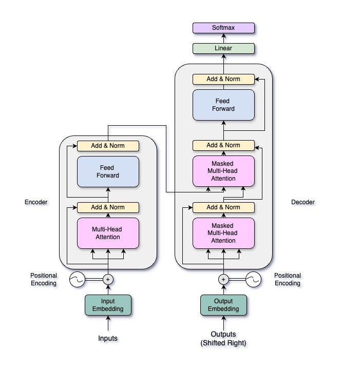
Transformer Architecture (Architecture in “Attention is all you need”) — Image by Author
A Transformer consists of two main parts: an encoder and a decoder. The encoder processes the input sequence to create a continuous representation, while the decoder generates the output sequence from this representation. Both the encoder and the decoder have multiple layers, each containing two essential components: a multi-head self-attention mechanism and a position-wise feed-forward network. In this article, we’ll focus on the multi-head attention mechanism, but we’ll explore the entire Transformer architecture in future articles.
1.2: Multi-Head Attention Overview
Multi-head attention enables the model to focus on different parts of the input sequence at the same time, capturing various aspects of the data. Think of it like having multiple spotlights shining on different parts of a stage. Each spotlight (or “head”) can illuminate a different performer (or data feature), allowing the audience (or model) to see the whole scene more clearly. By splitting the input into multiple subspaces, each with its attention mechanism, multi-head attention provides the model with several views of the input data. This setup helps the model understand complex relationships within the data more effectively.
This mechanism allows the Transformer to capture different relationships in the data by attending to various parts of the sequence. This improves the learning process by offering multiple perspectives of the input, enhancing the model’s ability to generalize. It also increases the model’s expressiveness by enabling it to learn different aspects of the input data simultaneously.
These capabilities make multi-head attention a crucial component in the success of Transformer models across a range of applications, from language translation to image processing.
2: The Mathematical Foundations
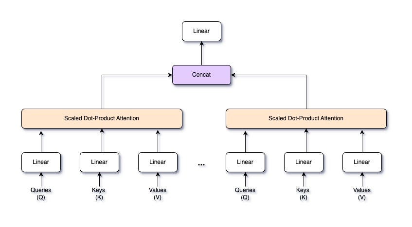
Multi-Head Attention Architecture — Image by Author
2.1: Attention Mechanism
The attention mechanism in neural networks is designed to mimic the human ability to focus on specific parts of information while processing data. Imagine reading a book: your eyes don’t pay equal attention to every word on the page. Instead, they focus more on the important words that help you understand the story. Similarly, in neural networks, attention allows the model to dynamically weigh the importance of different input elements. This means the model can prioritize parts of the input sequence that are more relevant for generating the output, improving its performance in tasks like language translation, text summarization, and more.
Mathematically, the attention mechanism can be described using a set of queries, keys, and values. Let’s denote the input as a set of queries Q, keys K, and values V. These are typically linear transformations of the input data.
The attention scores are calculated by taking the dot product of the query with all keys, which gives a measure of similarity. For a query q and a set of keys k1, k2, …, kn, the attention scores are given by:
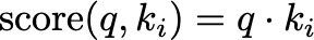
Attention Score — Image by Author
Think of this as comparing how similar each word (key) in a sentence is to the word (query) you’re focusing on. Higher scores indicate greater similarity.
To prevent the dot products from becoming too large, especially when dealing with high-dimensional vectors, we scale the scores by the square root of the dimension of the keys, d_k:
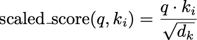
Scaled Score Formula — Image by Author
This is like adjusting the intensity of the spotlight based on how large the stage is. It ensures that the scores remain manageable and helps maintain stable gradients during training. This scaling ensures that the values passed to the softmax function have a standard deviation close to 1, which helps maintain stable gradients during training.
To see why this is necessary, consider the properties of dot products and high-dimensional vectors. When we compute the dot product of two vectors q and k_i of dimension d_k, the expected value of their dot product is proportional to d_k. Without scaling, as d_k increases, the variance of the dot product grows, leading to very large values which can cause the softmax function to produce near-binary outputs (i.e., probabilities close to 0 or 1). This sharpness reduces the model’s ability to learn effectively because it makes the gradients very small.
By dividing the dot product by d_k, we normalize the input to the softmax function, ensuring that the scores remain within a reasonable range. This normalization helps the model to maintain a balance, enabling it to learn more effectively and stably.
These scaled scores are then passed through a softmax function to obtain the attention weights. The softmax function converts the scores into probabilities, which represent the importance of each key relative to the query:
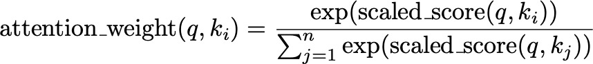
Attention Weight using Softmax Function — Image by Author
This step is like converting the adjusted spotlight intensities into a clear ranking, highlighting the most relevant parts of the scene more brightly.
The final attention output is obtained by taking a weighted sum of the values, using the attention weights:
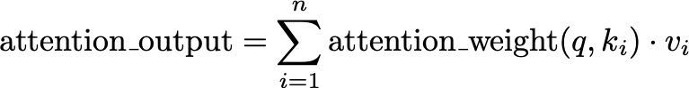
Attention Output Formula — Image by Author
Here, v_i represents the value corresponding to key k_i. This weighted sum combines the most relevant information from the values, much like focusing your attention on the most important parts of the book to understand the story better.
2.2: Multi-Head Attention
Multi-head attention is an advanced form of the attention mechanism that allows a model to focus on different parts of the input sequence simultaneously, capturing various relationships within the data. Instead of having a single attention mechanism, multi-head attention splits the input into multiple “heads,” each with its own set of queries, keys, and values. Each head performs the attention operation independently, and their outputs are then combined. This enhances the model’s ability to understand complex patterns and dependencies in the data.
Imagine you’re trying to understand a complex scene with many elements. If you had multiple pairs of eyes, each looking at different parts of the scene, you’d get a more comprehensive understanding. Similarly, multi-head attention allows the model to focus on different parts of the input data at once, providing a richer and more detailed representation.
Given an input sequence X, we project it into queries Q, keys K, and values V using learned linear transformations. For each head i, we have separate weight matrices W_Q, W_K, and W_V:

Queries, Keys, and Values Linear Transformations — Image by Author
These projections allow each head to focus on different aspects of the input data. For each head i, we compute the attention scores using the scaled dot-product attention mechanism. The attention output for head i is:
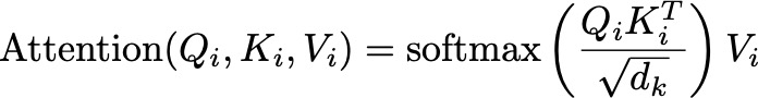
Attention Formula — Image by Author
Here, d_k is the dimension of the key vectors, ensuring the scores are appropriately scaled.
After computing the attention outputs for all heads, we concatenate them along the feature dimension. If we have h heads, each producing an output of dimension d_v, the concatenated output will have a dimension of h×d_v:

Multi-Head Concatenation — Image by Author
The concatenated output is then projected back to the original input dimension d using a learned weight matrix W_O:
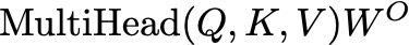
Final Layer of Multi-Head Attention — Image by Author
This final linear transformation combines the outputs from all heads into a single representation.
The core idea behind combining multiple attention heads is to allow the model to capture different types of information from the input sequence simultaneously. By having multiple heads, each head can learn to attend to different parts of the input or different features. This diversity in attention leads to a richer and more nuanced representation of the data.
2.3: Position-wise Feed-Forward Networks
In the Transformer architecture, each layer consists of a multi-head attention mechanism followed by a position-wise feed-forward network. These feed-forward layers are applied independently to each position in the sequence, hence the term “position-wise.” Essentially, they are simple fully connected neural networks applied separately and identically to each position of the input sequence.
Imagine a factory where every product on the conveyor belt goes through the same set of machines. Each machine processes the product in a specific way, adding something new or refining it. Similarly, each position in the sequence is processed independently by the feed-forward layers, transforming and enhancing the representation.
The purpose of these feed-forward layers is to introduce non-linearity and additional learning capacity to the model. After the attention mechanism has aggregated information from different parts of the sequence, the feed-forward network processes this information to further transform and refine the representation.
Mathematically, a position-wise feed-forward network consists of two linear transformations with a ReLU activation function in between. Given an input x at a particular position, the feed-forward network can be represented as:

Feed-Forward Network Formula — Image by Author
Here:
The input x is first linearly transformed using the weight matrix W1 and bias b1:
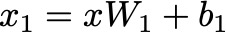
Linear Transformation of the input — Image by Author
Think of this step as passing the input through the first machine in the factory, which adds initial modifications based on learned weights and biases.
The linear transformation is followed by a ReLU activation function, which introduces non-linearity:
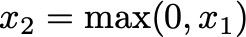
ReLU Formula — Image by Author
ReLU (Rectified Linear Unit) sets all negative values to zero, allowing the model to capture non-linear relationships in the data. This step is like ensuring only positive contributions from the first machine are passed on.
The activated output is then passed through a second linear transformation using weight matrix W2 and bias b2:
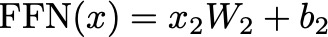
Second FFN — Image by Author
This final step further refines the output, much like the second machine in the factory making additional modifications to produce a finished product.
The position-wise feed-forward network in the Transformer architecture further processes the information captured by the multi-head attention mechanism. While the attention mechanism allows the model to focus on different parts of the sequence and aggregate context-specific information, the feed-forward network refines and transforms this information at each position. This enhances the model’s ability to capture complex patterns and dependencies.
3: Building Multi-Head Attention from Scratch
In this section, we will break down and explain the implementation of a multi-head attention mechanism from scratch using Python and numpy. The goal is to understand how the input is modified during the process. Before proceed with your reading, take a look at the code we will cover in this section. You should be able to get a general understanding, but don’t worry if now, as we will go over each line in this section.
models-from-scratch-python/Multi-Head Attention/demo.py at main · cristianleoo/models-from-scratch-python
To begin, we define the MultiHeadAttention class, which is responsible for managing the parameters needed for the multi-head attention mechanism. Let's go through this step-by-step to understand how we set it up.
import numpy
class MultiHeadAttention:
def __init__(self, num_hiddens, num_heads, dropout=0.0, bias=False):
self.num_heads = num_heads
self.num_hiddens = num_hiddens
self.d_k = self.d_v = num_hiddens // num_heads
In the initialization method, we first set the number of attention heads and the total number of hidden units in the model. These values are provided as arguments when the class is instantiated.
We then calculate the dimensions of the queries and values for each head. Since the total number of hidden units (num_hiddens) is split across all heads (num_heads), each head will have a query and value dimension of num_hiddens // num_heads.
self.W_q = np.random.rand(num_hiddens, num_hiddens)
self.W_k = np.random.rand(num_hiddens, num_hiddens)
self.W_v = np.random.rand(num_hiddens, num_hiddens)
self.W_o = np.random.rand(num_hiddens, num_hiddens)
Next, we initialize the weight matrices for the queries, keys, values, and output transformations. These weight matrices are randomly initialized:
if bias:
self.b_q = np.random.rand(num_hiddens)
self.b_k = np.random.rand(num_hiddens)
self.b_v = np.random.rand(num_hiddens)
self.b_o = np.random.rand(num_hiddens)
else:
self.b_q = self.b_k = self.b_v = self.b_o = np.zeros(num_hiddens)
Finally, we initialize the bias vectors for the queries, keys, values, and output transformations. If the bias parameter is set to True, these biases are randomly initialized. Otherwise, they are set to zero:
The biases have dimensions equal to the number of hidden units, num_hiddens.
By setting up these weights and biases, we ensure that each attention head can independently learn to focus on different parts of the input data.
Next, we define methods to prepare and transform the data for multi-head attention. First, let’s look at the transpose_qkv method:
def transpose_qkv(self, X):
X = X.reshape(X.shape[0], X.shape[1], self.num_heads, -1)
X = X.transpose(0, 2, 1, 3)
return X.reshape(-1, X.shape[2], X.shape[3])
This method is responsible for reshaping and transposing the input data to prepare it for multi-head attention. In particular:
X = X.reshape(X.shape[0], X.shape[1], self.num_heads, -1)
This line reshapes the input tensor X to have four dimensions: (batch_size, sequence_length, num_heads, depth_per_head).
X = X.transpose(0, 2, 1, 3)
This line transposes the tensor so that the dimensions are reordered to (batch_size, num_heads, sequence_length, depth_per_head).
This rearrangement ensures that each attention head processes its part of the input sequence independently.
return X.reshape(-1, X.shape[2], X.shape[3])
This final reshape flattens the batch and head dimensions into a single dimension, resulting in a tensor of shape (batch_size * num_heads, sequence_length, depth_per_head).
By doing this, transpose_qkv ensures that the input data is split correctly among the multiple heads, with each head having the appropriate dimensions to process its segment of the data.
Next, we have the transpose_output method:
def transpose_output(self, X):
X = X.reshape(-1, self.num_heads, X.shape[1], X.shape[2])
X = X.transpose(0, 2, 1, 3)
return X.reshape(X.shape[0], X.shape[1], -1)
This method reverses the transformation done by transpose_qkv to combine the outputs from all heads back into the original shape.
After transposing our matrices, we can process with the scaled dot-product attention mechanism, which allows the model to focus on different parts of the input sequence with varying degrees of importance.
def scaled_dot_product_attention(self, Q, K, V, valid_lens):
d_k = Q.shape[-1]
scores = np.matmul(Q, K.transpose(0, 2, 1)) / np.sqrt(d_k)
if valid_lens is not None:
mask = np.arange(scores.shape[-1]) < valid_lens[:, None]
scores = np.where(mask[:, None, :], scores, -np.inf)
attention_weights = np.exp(scores - np.max(scores, axis=-1, keepdims=True))
attention_weights /= attention_weights.sum(axis=-1, keepdims=True)
return np.matmul(attention_weights, V)
The inputs to this method are the query (Q), key (K), and value (V) matrices. These matrices are derived from the input data through linear transformations.
d_k = Q.shape[-1]
Here, we extract the dimension of the key vectors, d_k, from the last dimension of the query matrix Q. This value is used for scaling the attention scores.
scores = np.matmul(Q, K.transpose(0, 2, 1)) / np.sqrt(d_k)
We calculate the attention scores by performing a matrix multiplication of Q and the transpose of K. The scores are then scaled by the square root of d_k. This scaling helps prevent the scores from growing too large, which can lead to issues during the softmax calculation.
Next, we define the forward pass method to process the input data through the multi-head attention mechanism. This method is crucial as it orchestrates the entire multi-head attention process, from transforming the input data to combining the outputs from multiple heads.
def forward(self, queries, keys, values, valid_lens):
queries = self.transpose_qkv(np.dot(queries, self.W_q) + self.b_q)
keys = self.transpose_qkv(np.dot(keys, self.W_k) + self.b_k)
values = self.transpose_qkv(np.dot(values, self.W_v) + self.b_v)
if valid_lens is not None:
valid_lens = np.repeat(valid_lens, self.num_heads, axis=0)
output = self.scaled_dot_product_attention(queries, keys, values, valid_lens)
output_concat = self.transpose_output(output)
return np.dot(output_concat, self.W_o) + self.b_o
Let’s break down the forward method:
queries = self.transpose_qkv(np.dot(queries, self.W_q) + self.b_q)
keys = self.transpose_qkv(np.dot(keys, self.W_k) + self.b_k)
values = self.transpose_qkv(np.dot(values, self.W_v) + self.b_v)
First, the input queries, keys, and values are projected into their respective subspaces using the learned weight matrices (W_q, W_k, W_v) and biases (b_q, b_k, b_v). This is done by performing matrix multiplication with the weight matrices and adding the biases. The results are then transformed for multi-head attention using the transpose_qkv method, which reshapes and transposes the data to ensure each head processes the input independently.
Queries, keys, and values are the transformed inputs, now prepared for multi-head attention.
if valid_lens is not None:
valid_lens = np.repeat(valid_lens, self.num_heads, axis=0)
If valid_lens (valid lengths) are provided, they are repeated for each head. This ensures that the appropriate mask is created for each attention head, allowing the model to focus only on valid positions within the sequences.
output = self.scaled_dot_product_attention(queries, keys, values, valid_lens)
The method then calls scaled_dot_product_attention with the transformed queries, keys, values, and repeated valid lengths. This function calculates the attention scores, applies the softmax function to obtain attention weights, and computes the weighted sum of the values to produce the attention output for each head.
output_concat = self.transpose_output(output)
return np.dot(output_concat, self.W_o) + self.b_o
After obtaining the attention outputs from all heads, the method concatenates these outputs along the feature dimension using transpose_output. This method reverses the initial transformation, combining the outputs from all heads back into a single representation. The concatenated output is then transformed back to the original input dimension using a final linear transformation with weight matrix W_o and bias b_o.
Lastly, we test the class with some sample data. Here’s how we do it:
# Define dimensions and initialize multi-head attention
num_hiddens, num_heads = 100, 5
attention = MultiHeadAttention(num_hiddens, num_heads, dropout=0.5, bias=False)
We initialize the MultiHeadAttention class with 100 hidden units and 5 attention heads. This sets up the necessary parameters and weight matrices for the multi-head attention mechanism.
# Define sample data
batch_size, num_queries, num_kvpairs = 2, 4, 6
valid_lens = np.array([3, 2])
X = np.random.rand(batch_size, num_queries, num_hiddens) # Use random data to simulate input queries
Y = np.random.rand(batch_size, num_kvpairs, num_hiddens) # Use random data to simulate key-value pairs
We create random data to simulate input queries (X) and key-value pairs (Y). The batch size is 2, the number of queries is 4, and the number of key-value pairs is 6. We also define valid lengths (valid_lens) to indicate the valid positions within the sequences.
# Apply multi-head attention
output = attention.forward(X, Y, Y, valid_lens)
We pass the sample data through the multi-head attention mechanism using the forward method. This processes the input queries, keys, and values, applying the multi-head attention calculations.
print("Output shape:", output.shape)
# Output should be: (2, 4, 100)
print("Output data:", output)
We print the shape and content of the output. The expected output shape ensures that the output dimensions match the original input dimensions. Then, we print the output data after computing Multi-Head Attention. Now that you have an understanding of how the Multi-Head Attention mechanism works, try tweaking it. For instance, change the number of heads, try adding multiple FFN before and after Multi-Head Attention. Also, you could try to implement it in a machine translation task, and see it in action. Let me know if you would like me to do that in a next article.
Conclusion
Transformers have transformed deep learning, especially in NLP, by using self-attention mechanisms that allow for parallel processing of input sequences. This approach not only speeds up computation but also handles long-range dependencies more effectively than traditional recurrent neural networks).
In this article, we’ve gained a comprehensive understanding of multi-head attention in Transformers, from it’s math theory to a practical code implementation. Maybe for now the concepts we will still be abstracts, as you can’t really do anything with the outputs from Multi-Head Attention, but soon we will see how they play a key role in the transformer architecture, which is the base of the well-known LLMs around (Claude, ChatGPT, …). Stay tuned for future articles, where we’ll explore the remaining components of the Transformer architecture, offering deeper insights into this powerful model.
References

The Math Behind Multi-Head Attention in Transformers was originally published in Towards Data Science on Medium, where people are continuing the conversation by highlighting and responding to this story.
Image generated by DALL-E
1: Introduction
1.1: Transformers Overview
The Transformer architecture, introduced by Vaswani et al. in their paper “Attention is All You Need” has transformed deep learning, particularly in natural language processing (NLP). Transformers use a self-attention mechanism, enabling them to handle input sequences all at once. This parallel processing allows for faster computation and better management of long-range dependencies within the data. This doesn’t sound familiar? Don’t worry as it will be at the end of this article. Let’s first take a brief look at what a Transformer looks like.
Transformer Architecture (Architecture in “Attention is all you need”) — Image by Author
A Transformer consists of two main parts: an encoder and a decoder. The encoder processes the input sequence to create a continuous representation, while the decoder generates the output sequence from this representation. Both the encoder and the decoder have multiple layers, each containing two essential components: a multi-head self-attention mechanism and a position-wise feed-forward network. In this article, we’ll focus on the multi-head attention mechanism, but we’ll explore the entire Transformer architecture in future articles.
1.2: Multi-Head Attention Overview
Multi-head attention enables the model to focus on different parts of the input sequence at the same time, capturing various aspects of the data. Think of it like having multiple spotlights shining on different parts of a stage. Each spotlight (or “head”) can illuminate a different performer (or data feature), allowing the audience (or model) to see the whole scene more clearly. By splitting the input into multiple subspaces, each with its attention mechanism, multi-head attention provides the model with several views of the input data. This setup helps the model understand complex relationships within the data more effectively.
This mechanism allows the Transformer to capture different relationships in the data by attending to various parts of the sequence. This improves the learning process by offering multiple perspectives of the input, enhancing the model’s ability to generalize. It also increases the model’s expressiveness by enabling it to learn different aspects of the input data simultaneously.
These capabilities make multi-head attention a crucial component in the success of Transformer models across a range of applications, from language translation to image processing.
2: The Mathematical Foundations
Multi-Head Attention Architecture — Image by Author
2.1: Attention Mechanism
The attention mechanism in neural networks is designed to mimic the human ability to focus on specific parts of information while processing data. Imagine reading a book: your eyes don’t pay equal attention to every word on the page. Instead, they focus more on the important words that help you understand the story. Similarly, in neural networks, attention allows the model to dynamically weigh the importance of different input elements. This means the model can prioritize parts of the input sequence that are more relevant for generating the output, improving its performance in tasks like language translation, text summarization, and more.
Mathematically, the attention mechanism can be described using a set of queries, keys, and values. Let’s denote the input as a set of queries Q, keys K, and values V. These are typically linear transformations of the input data.
The attention scores are calculated by taking the dot product of the query with all keys, which gives a measure of similarity. For a query q and a set of keys k1, k2, …, kn, the attention scores are given by:
Attention Score — Image by Author
Think of this as comparing how similar each word (key) in a sentence is to the word (query) you’re focusing on. Higher scores indicate greater similarity.
To prevent the dot products from becoming too large, especially when dealing with high-dimensional vectors, we scale the scores by the square root of the dimension of the keys, d_k:
Scaled Score Formula — Image by Author
This is like adjusting the intensity of the spotlight based on how large the stage is. It ensures that the scores remain manageable and helps maintain stable gradients during training. This scaling ensures that the values passed to the softmax function have a standard deviation close to 1, which helps maintain stable gradients during training.
To see why this is necessary, consider the properties of dot products and high-dimensional vectors. When we compute the dot product of two vectors q and k_i of dimension d_k, the expected value of their dot product is proportional to d_k. Without scaling, as d_k increases, the variance of the dot product grows, leading to very large values which can cause the softmax function to produce near-binary outputs (i.e., probabilities close to 0 or 1). This sharpness reduces the model’s ability to learn effectively because it makes the gradients very small.
By dividing the dot product by d_k, we normalize the input to the softmax function, ensuring that the scores remain within a reasonable range. This normalization helps the model to maintain a balance, enabling it to learn more effectively and stably.
These scaled scores are then passed through a softmax function to obtain the attention weights. The softmax function converts the scores into probabilities, which represent the importance of each key relative to the query:
Attention Weight using Softmax Function — Image by Author
This step is like converting the adjusted spotlight intensities into a clear ranking, highlighting the most relevant parts of the scene more brightly.
The final attention output is obtained by taking a weighted sum of the values, using the attention weights:
Attention Output Formula — Image by Author
Here, v_i represents the value corresponding to key k_i. This weighted sum combines the most relevant information from the values, much like focusing your attention on the most important parts of the book to understand the story better.
2.2: Multi-Head Attention
Multi-head attention is an advanced form of the attention mechanism that allows a model to focus on different parts of the input sequence simultaneously, capturing various relationships within the data. Instead of having a single attention mechanism, multi-head attention splits the input into multiple “heads,” each with its own set of queries, keys, and values. Each head performs the attention operation independently, and their outputs are then combined. This enhances the model’s ability to understand complex patterns and dependencies in the data.
Imagine you’re trying to understand a complex scene with many elements. If you had multiple pairs of eyes, each looking at different parts of the scene, you’d get a more comprehensive understanding. Similarly, multi-head attention allows the model to focus on different parts of the input data at once, providing a richer and more detailed representation.
Given an input sequence X, we project it into queries Q, keys K, and values V using learned linear transformations. For each head i, we have separate weight matrices W_Q, W_K, and W_V:
Queries, Keys, and Values Linear Transformations — Image by Author
These projections allow each head to focus on different aspects of the input data. For each head i, we compute the attention scores using the scaled dot-product attention mechanism. The attention output for head i is:
Attention Formula — Image by Author
Here, d_k is the dimension of the key vectors, ensuring the scores are appropriately scaled.
After computing the attention outputs for all heads, we concatenate them along the feature dimension. If we have h heads, each producing an output of dimension d_v, the concatenated output will have a dimension of h×d_v:
Multi-Head Concatenation — Image by Author
The concatenated output is then projected back to the original input dimension d using a learned weight matrix W_O:
Final Layer of Multi-Head Attention — Image by Author
This final linear transformation combines the outputs from all heads into a single representation.
The core idea behind combining multiple attention heads is to allow the model to capture different types of information from the input sequence simultaneously. By having multiple heads, each head can learn to attend to different parts of the input or different features. This diversity in attention leads to a richer and more nuanced representation of the data.
2.3: Position-wise Feed-Forward Networks
In the Transformer architecture, each layer consists of a multi-head attention mechanism followed by a position-wise feed-forward network. These feed-forward layers are applied independently to each position in the sequence, hence the term “position-wise.” Essentially, they are simple fully connected neural networks applied separately and identically to each position of the input sequence.
Imagine a factory where every product on the conveyor belt goes through the same set of machines. Each machine processes the product in a specific way, adding something new or refining it. Similarly, each position in the sequence is processed independently by the feed-forward layers, transforming and enhancing the representation.
The purpose of these feed-forward layers is to introduce non-linearity and additional learning capacity to the model. After the attention mechanism has aggregated information from different parts of the sequence, the feed-forward network processes this information to further transform and refine the representation.
Mathematically, a position-wise feed-forward network consists of two linear transformations with a ReLU activation function in between. Given an input x at a particular position, the feed-forward network can be represented as:
Feed-Forward Network Formula — Image by Author
Here:
- W1 and W2 are learned weight matrices.
- b1 and b2 are learned bias vectors.
- max(0, xW1+b1) represents the ReLU activation function applied element-wise.
The input x is first linearly transformed using the weight matrix W1 and bias b1:
Linear Transformation of the input — Image by Author
Think of this step as passing the input through the first machine in the factory, which adds initial modifications based on learned weights and biases.
The linear transformation is followed by a ReLU activation function, which introduces non-linearity:
ReLU Formula — Image by Author
ReLU (Rectified Linear Unit) sets all negative values to zero, allowing the model to capture non-linear relationships in the data. This step is like ensuring only positive contributions from the first machine are passed on.
The activated output is then passed through a second linear transformation using weight matrix W2 and bias b2:
Second FFN — Image by Author
This final step further refines the output, much like the second machine in the factory making additional modifications to produce a finished product.
The position-wise feed-forward network in the Transformer architecture further processes the information captured by the multi-head attention mechanism. While the attention mechanism allows the model to focus on different parts of the sequence and aggregate context-specific information, the feed-forward network refines and transforms this information at each position. This enhances the model’s ability to capture complex patterns and dependencies.
3: Building Multi-Head Attention from Scratch
In this section, we will break down and explain the implementation of a multi-head attention mechanism from scratch using Python and numpy. The goal is to understand how the input is modified during the process. Before proceed with your reading, take a look at the code we will cover in this section. You should be able to get a general understanding, but don’t worry if now, as we will go over each line in this section.
models-from-scratch-python/Multi-Head Attention/demo.py at main · cristianleoo/models-from-scratch-python
To begin, we define the MultiHeadAttention class, which is responsible for managing the parameters needed for the multi-head attention mechanism. Let's go through this step-by-step to understand how we set it up.
import numpy
class MultiHeadAttention:
def __init__(self, num_hiddens, num_heads, dropout=0.0, bias=False):
self.num_heads = num_heads
self.num_hiddens = num_hiddens
self.d_k = self.d_v = num_hiddens // num_heads
In the initialization method, we first set the number of attention heads and the total number of hidden units in the model. These values are provided as arguments when the class is instantiated.
- num_hiddens: This represents the total number of hidden units in the model. It's a crucial parameter because it determines the size of the linear transformations applied to the input data.
- num_heads: This indicates the number of attention heads. Each head will independently learn to focus on different parts of the input, enabling the model to capture various aspects of the data.
- dropout: This is the dropout rate, which is not used in this particular implementation but is included for completeness.
- bias: This is a boolean flag indicating whether to include biased terms in the linear transformations.
We then calculate the dimensions of the queries and values for each head. Since the total number of hidden units (num_hiddens) is split across all heads (num_heads), each head will have a query and value dimension of num_hiddens // num_heads.
self.W_q = np.random.rand(num_hiddens, num_hiddens)
self.W_k = np.random.rand(num_hiddens, num_hiddens)
self.W_v = np.random.rand(num_hiddens, num_hiddens)
self.W_o = np.random.rand(num_hiddens, num_hiddens)
Next, we initialize the weight matrices for the queries, keys, values, and output transformations. These weight matrices are randomly initialized:
- W_q is used to transform the input data into queries. It has dimensions num_hiddens x num_hiddens, meaning it maps the input features to the query space.
- W_k is used to transform the input data into keys. It also has dimensions num_hiddens x num_hiddens, mapping the input features to the key space.
- W_v is used to transform the input data into values, with the same dimensions as the previous matrices.
- W_o is used to transform the concatenated output of all heads back to the original input dimensions.
if bias:
self.b_q = np.random.rand(num_hiddens)
self.b_k = np.random.rand(num_hiddens)
self.b_v = np.random.rand(num_hiddens)
self.b_o = np.random.rand(num_hiddens)
else:
self.b_q = self.b_k = self.b_v = self.b_o = np.zeros(num_hiddens)
Finally, we initialize the bias vectors for the queries, keys, values, and output transformations. If the bias parameter is set to True, these biases are randomly initialized. Otherwise, they are set to zero:
- b_q: Bias for the query transformation.
- b_k: Bias for the key transformation.
- b_v: Bias for the value transformation.
- b_o: Bias for the output transformation.
The biases have dimensions equal to the number of hidden units, num_hiddens.
By setting up these weights and biases, we ensure that each attention head can independently learn to focus on different parts of the input data.
Next, we define methods to prepare and transform the data for multi-head attention. First, let’s look at the transpose_qkv method:
def transpose_qkv(self, X):
X = X.reshape(X.shape[0], X.shape[1], self.num_heads, -1)
X = X.transpose(0, 2, 1, 3)
return X.reshape(-1, X.shape[2], X.shape[3])
This method is responsible for reshaping and transposing the input data to prepare it for multi-head attention. In particular:
X = X.reshape(X.shape[0], X.shape[1], self.num_heads, -1)
This line reshapes the input tensor X to have four dimensions: (batch_size, sequence_length, num_heads, depth_per_head).
- X.shape[0] is the batch size.
- X.shape[1] is the sequence length (number of positions in the input sequence).
- self.num_heads is the number of attention heads.
- -1 automatically infers the size of the last dimension (depth per head) so that the total number of elements remains the same.
X = X.transpose(0, 2, 1, 3)
This line transposes the tensor so that the dimensions are reordered to (batch_size, num_heads, sequence_length, depth_per_head).
This rearrangement ensures that each attention head processes its part of the input sequence independently.
return X.reshape(-1, X.shape[2], X.shape[3])
This final reshape flattens the batch and head dimensions into a single dimension, resulting in a tensor of shape (batch_size * num_heads, sequence_length, depth_per_head).
By doing this, transpose_qkv ensures that the input data is split correctly among the multiple heads, with each head having the appropriate dimensions to process its segment of the data.
Next, we have the transpose_output method:
def transpose_output(self, X):
X = X.reshape(-1, self.num_heads, X.shape[1], X.shape[2])
X = X.transpose(0, 2, 1, 3)
return X.reshape(X.shape[0], X.shape[1], -1)
This method reverses the transformation done by transpose_qkv to combine the outputs from all heads back into the original shape.
After transposing our matrices, we can process with the scaled dot-product attention mechanism, which allows the model to focus on different parts of the input sequence with varying degrees of importance.
def scaled_dot_product_attention(self, Q, K, V, valid_lens):
d_k = Q.shape[-1]
scores = np.matmul(Q, K.transpose(0, 2, 1)) / np.sqrt(d_k)
if valid_lens is not None:
mask = np.arange(scores.shape[-1]) < valid_lens[:, None]
scores = np.where(mask[:, None, :], scores, -np.inf)
attention_weights = np.exp(scores - np.max(scores, axis=-1, keepdims=True))
attention_weights /= attention_weights.sum(axis=-1, keepdims=True)
return np.matmul(attention_weights, V)
The inputs to this method are the query (Q), key (K), and value (V) matrices. These matrices are derived from the input data through linear transformations.
d_k = Q.shape[-1]
Here, we extract the dimension of the key vectors, d_k, from the last dimension of the query matrix Q. This value is used for scaling the attention scores.
scores = np.matmul(Q, K.transpose(0, 2, 1)) / np.sqrt(d_k)
We calculate the attention scores by performing a matrix multiplication of Q and the transpose of K. The scores are then scaled by the square root of d_k. This scaling helps prevent the scores from growing too large, which can lead to issues during the softmax calculation.
Next, we define the forward pass method to process the input data through the multi-head attention mechanism. This method is crucial as it orchestrates the entire multi-head attention process, from transforming the input data to combining the outputs from multiple heads.
def forward(self, queries, keys, values, valid_lens):
queries = self.transpose_qkv(np.dot(queries, self.W_q) + self.b_q)
keys = self.transpose_qkv(np.dot(keys, self.W_k) + self.b_k)
values = self.transpose_qkv(np.dot(values, self.W_v) + self.b_v)
if valid_lens is not None:
valid_lens = np.repeat(valid_lens, self.num_heads, axis=0)
output = self.scaled_dot_product_attention(queries, keys, values, valid_lens)
output_concat = self.transpose_output(output)
return np.dot(output_concat, self.W_o) + self.b_o
Let’s break down the forward method:
queries = self.transpose_qkv(np.dot(queries, self.W_q) + self.b_q)
keys = self.transpose_qkv(np.dot(keys, self.W_k) + self.b_k)
values = self.transpose_qkv(np.dot(values, self.W_v) + self.b_v)
First, the input queries, keys, and values are projected into their respective subspaces using the learned weight matrices (W_q, W_k, W_v) and biases (b_q, b_k, b_v). This is done by performing matrix multiplication with the weight matrices and adding the biases. The results are then transformed for multi-head attention using the transpose_qkv method, which reshapes and transposes the data to ensure each head processes the input independently.
Queries, keys, and values are the transformed inputs, now prepared for multi-head attention.
if valid_lens is not None:
valid_lens = np.repeat(valid_lens, self.num_heads, axis=0)
If valid_lens (valid lengths) are provided, they are repeated for each head. This ensures that the appropriate mask is created for each attention head, allowing the model to focus only on valid positions within the sequences.
output = self.scaled_dot_product_attention(queries, keys, values, valid_lens)
The method then calls scaled_dot_product_attention with the transformed queries, keys, values, and repeated valid lengths. This function calculates the attention scores, applies the softmax function to obtain attention weights, and computes the weighted sum of the values to produce the attention output for each head.
output_concat = self.transpose_output(output)
return np.dot(output_concat, self.W_o) + self.b_o
After obtaining the attention outputs from all heads, the method concatenates these outputs along the feature dimension using transpose_output. This method reverses the initial transformation, combining the outputs from all heads back into a single representation. The concatenated output is then transformed back to the original input dimension using a final linear transformation with weight matrix W_o and bias b_o.
Lastly, we test the class with some sample data. Here’s how we do it:
# Define dimensions and initialize multi-head attention
num_hiddens, num_heads = 100, 5
attention = MultiHeadAttention(num_hiddens, num_heads, dropout=0.5, bias=False)
We initialize the MultiHeadAttention class with 100 hidden units and 5 attention heads. This sets up the necessary parameters and weight matrices for the multi-head attention mechanism.
# Define sample data
batch_size, num_queries, num_kvpairs = 2, 4, 6
valid_lens = np.array([3, 2])
X = np.random.rand(batch_size, num_queries, num_hiddens) # Use random data to simulate input queries
Y = np.random.rand(batch_size, num_kvpairs, num_hiddens) # Use random data to simulate key-value pairs
We create random data to simulate input queries (X) and key-value pairs (Y). The batch size is 2, the number of queries is 4, and the number of key-value pairs is 6. We also define valid lengths (valid_lens) to indicate the valid positions within the sequences.
# Apply multi-head attention
output = attention.forward(X, Y, Y, valid_lens)
We pass the sample data through the multi-head attention mechanism using the forward method. This processes the input queries, keys, and values, applying the multi-head attention calculations.
print("Output shape:", output.shape)
# Output should be: (2, 4, 100)
print("Output data:", output)
We print the shape and content of the output. The expected output shape ensures that the output dimensions match the original input dimensions. Then, we print the output data after computing Multi-Head Attention. Now that you have an understanding of how the Multi-Head Attention mechanism works, try tweaking it. For instance, change the number of heads, try adding multiple FFN before and after Multi-Head Attention. Also, you could try to implement it in a machine translation task, and see it in action. Let me know if you would like me to do that in a next article.
Conclusion
Transformers have transformed deep learning, especially in NLP, by using self-attention mechanisms that allow for parallel processing of input sequences. This approach not only speeds up computation but also handles long-range dependencies more effectively than traditional recurrent neural networks).
In this article, we’ve gained a comprehensive understanding of multi-head attention in Transformers, from it’s math theory to a practical code implementation. Maybe for now the concepts we will still be abstracts, as you can’t really do anything with the outputs from Multi-Head Attention, but soon we will see how they play a key role in the transformer architecture, which is the base of the well-known LLMs around (Claude, ChatGPT, …). Stay tuned for future articles, where we’ll explore the remaining components of the Transformer architecture, offering deeper insights into this powerful model.
References
- Vaswani, A., Shazeer, N., Parmar, N., Uszkoreit, J., Jones, L., Gomez, A. N., Kaiser, Ł., & Polosukhin, I. (2017). Attention is All You Need. In Advances in Neural Information Processing Systems (NeurIPS).
- Alammar, J. (2018). The Illustrated Transformer. jalammar.github.io.
The Math Behind Multi-Head Attention in Transformers was originally published in Towards Data Science on Medium, where people are continuing the conversation by highlighting and responding to this story.