A powerful yet under-the-radar method for data summarization and explainable AI
Despite being a powerful tool for data summarization, the MMD-Critic method has a surprising lack of both usage and “coverage”. Perhaps this is because simpler and more established methods for data summarization exist (e.g. K-medoids, see [1] or, more simply, the Wikipedia page), or perhaps this is because no Python package for the method existed (before now). Regardless, the results presented in the original paper [2] warrant more use than MMD-Critic has currently. As such, I’ll explain the MMD-Critic method here with as much clarity as possible. I’ve also published an open-source Python package with an implementation of the technique so you can use it easily.
Prototypes and Criticisms
Before jumping into the MMD-Critic method itself, it’s worth discussing what exactly we’re trying to accomplish. Ultimately, we wish to take a dataset and find examples that are representative of the data (prototypes), as well as edge-case examples that may confound our machine learning models (criticisms).
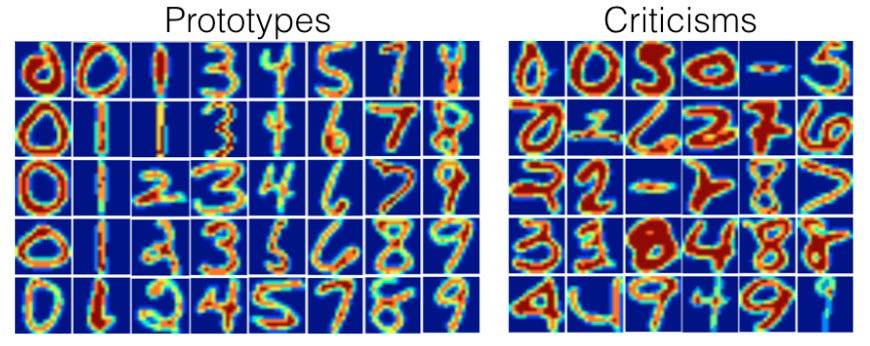
Prototypes and criticisms for the MNIST dataset, taken from [2].
There are many reasons why this may be useful:
You can see section 6.3 in this book for more info on the applications of this (and for a decent explanation of MMD-Critic as well), but it suffices to say that finding these examples is useful for a wide variety of reasons. MMD-Critic allows us to do this.
Maximal Mean Discrepancy
I unfortunately cannot claim to have a hyper-rigorous understanding of Maximal Mean Discrepancy (MMD), as such an understanding would require a strong background in functional analysis. If you have such a background, you can find the paper that introduced the measure here.
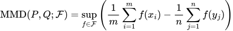
In simple terms though, MMD is a way to determine the difference between two probability distributions. Formally, for two probability distributions P and Q, we define the MMD of the two as

The formula for the MMD of two distributions P, Q
Here, F is any function space — that is, any set of functions with the same domain and codomain. Note also that the notation x~P means that we are treating x as if it’s a random variable drawn from the distribution P — that is, x is described by P. This formula thus finds the highest difference in the expected values of X and Y when they are transformed by some function from our space F.
This may be a little hard to wrap your head around, but here’s an example. Suppose that X is Uniform(0, 1) (i.e. a distribution that is equivalent to picking a random number from 0 to 1), and Y is Uniform(-1, 1) . Let’s also let F be a fairly simple family containing three functions — f(x) = 0, f(x) = x, and f(x) = x². Iterating over each function in our space, we get:
Formula for the expected value of a random variable x transformed by a function f
thus in the P case, we get
Expected value of f(x) under the distribution P
and in the Q case, we get
Expected value of f(x) under the distribution Q
thus our discrepancy in this case is also 0. The supremum over our function space is thus 0.5, so that’s our MMD.
You may now notice a few problems with our MMD. It seems highly dependent on our choice of function space and also appears highly expensive (or even impossible) to compute for a large or infinite function space. Not only that, but it also requires us to know our distributions P and Q, which is not realistic.
The latter problem is easily solvable, as we can rewrite our MMD metric to use estimates of P and Q based on our dataset:
MMD using estimates of P and Q
Here, our x’s are our samples from the dataset drawing from P, and the y’s are the samples drawn from Q.
The first two problems are solvable with a bit of extra math. Without going into too much detail, it turns out that if F is something called a Reproducing Kernel Hilbert Space (RKHS), we know what function is going to give us our MMD in advance. Namely, it’s the following function, called the witness function:

Our optimal f(x) in an RKHS
where k is the kernel (inner product) associated with the RKHS¹. Intuitively, this function “witnesses” the discrepancy between P and Q at the point x.
We thus only need to choose a sufficiently expressive RKHS/kernel — usually, the RBF kernel is used which has the kernel function
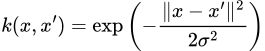
The RBF kernel, where sigma is a hyperparameter
This generally gets fairly intuitive results. Here, for instance, is the plot of the witness function with the RBF kernel when estimated (in the same way as mentioned before — that is, replacing expectations with a sum) on two datasets drawn from Uniform(-0.5, 0.5) and Uniform(-1, 1) :
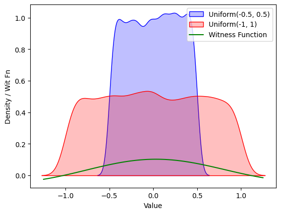
Values of the witness function at different points for two uniform distributions
The code for generating the above graph is here:
import numpy as np
import matplotlib.pyplot as plt
import seaborn as sns
def rbf(v1, v2, sigma=0.5):
return np.exp(-(v2 - v1) ** 2/(2 * sigma**0.5))
def comp_wit_fn(x, d1, d2):
return 1/len(d1) * sum([rbf(x, dp) for dp in d1]) - 1/len(d2) * sum([rbf(x, dp) for dp in d2])
low1, high1 = -0.5, 0.5 # Range for the first uniform distribution
low2, high2 = -1, 1 # Range for the second uniform distribution
# Generate data for the uniform distributions
data1 = np.random.uniform(low1, high1, 10000)
data2 = np.random.uniform(low2, high2, 10000)
# Generate a range of x values for which to compute comp_wit_fn
x_values = np.linspace(min(low1 * 2, low2 * 2), max(high1 * 2, high2 * 2), 100)
comp_wit_values = [comp_wit_fn(x, data1, data2) for x in x_values]
sns.kdeplot(data1, label=f'Uniform({low1}, {high1})', color='blue', fill=True)
sns.kdeplot(data2, label=f'Uniform({low2}, {high2})', color='red', fill=True)
plt.plot(x_values, comp_wit_values, label='Witness Function', color='green')
plt.xlabel('Value')
plt.ylabel('Density / Wit Fn')
plt.legend()
plt.show()
The MMD-Critic Method, Finally
The idea behind MMD-Critic is now fairly simple — if we want to find k prototypes, we need to find the set of prototypes that best matches the distribution of the original dataset given by their squared MMD. In other words, we wish to find a subset P of cardinality k of our dataset that minimizes MMD²(F, X, P). Without going into too much detail about why, the square MMD is given by
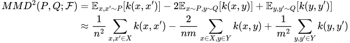
The square MMD metric, with X ~ P, Y ~ Q, and k the kernel for our RKHS F
After finding these prototypes, we then select the points where the hypothetical distribution of our prototypes is most different from our dataset distribution as criticisms. As we’ve seen before, the difference between two distributions at a point can be measured by our witness function, so we just find points that maximize its absolute value in the context of X and P. In other words, we define our criticism “score” as

The “score” for a criticism c
Or, in the more usable approximate form,
The approximated S(c) for a criticism c
Then, to find our desired amount of criticisms, say m of them, we simply wish to find the set C of size m that maximizes

To promote picking more varied criticisms, the paper also suggests adding a regularizer term that encourages selected criticisms to be as far apart as possible. The suggested regularizer in the paper is the log determinant regularizer, though this is not required. I won’t go into much detail here since it’s not critical, but the paper suggests reading [6]².
We can thus implement an extremely naive MMD-Critic without criticism regularization as follows (do NOT use this):
import math
import itertools
def euc_distance(p1, p2):
return math.sqrt(sum((x - y) ** 2 for x, y in zip(p1, p2)))
def rbf(v1, v2, sigma=0.5):
return math.exp(-euc_distance(v1, v2) ** 2/(2 * sigma**0.5))
def mmd_sq(X, Y, sigma=0.5):
sm_xx = 0
for x in X:
for x2 in X:
sm_xx += rbf(x, x2, sigma)
sm_xy = 0
for x in X:
for y in Y:
sm_xy += rbf(x, y, sigma)
sm_yy = 0
for y in Y:
for y2 in Y:
sm_yy += rbf(y, y2, sigma)
return 1/(len(X) ** 2) * sm_xx \
- 2/(len(X) * len(Y)) * sm_xy \
+ 1/(len(Y) ** 2) * sm_yy
def select_protos(X, n, sigma=0.5):
min_score, min_sub = math.inf, None
for subset in itertools.combinations(X, n):
new_mmd = mmd_sq(X, subset, sigma)
if new_mmd < min_score:
min_score = new_mmd
min_sub = subset
return min_sub
def criticism_score(criticism, prototypes, X, sigma=0.5):
return abs(1/len(X) * sum([rbf(criticism, x, sigma) for x in X])\
- 1/len(prototypes) * sum([rbf(criticism, p, sigma) for p in prototypes]))
def select_criticisms(X, P, n, sigma=0.5):
candidates = [c for c in X if c not in P]
max_score, crits = -math.inf, []
for subset in itertools.combinations(candidates, n):
new_score = sum([criticism_score(c, P, X, sigma) for c in subset])
if new_score > max_score:
max_score = new_score
crits = subset
return crits
Optimizing MMD-Critic
The above implementation is so impractical that, when I ran it, I failed to find 5 prototypes in a dataset with 25 points in a reasonable time. This is because our MMD calculation is O(max(|X|, |Y|)²), and iterating over every length-n subset is O(C(|X|, n)) (where C is the choose function), which gives us a horrendous runtime complexity.
Disregarding using more efficient computation methods (e.g. using pure numpy/numexpr/matrix calculations instead of loops/whatever) and caching repeated calculations, there are a few optimizations we can make on the theoretical level. Firstly, the most obvious slowdown we have is looping over the C(|X|, n) subsets in our prototype and criticism methods. Instead of that, we can use an approximation that loops n times, greedily selecting the best prototype each time. This allows us to change our prototype selection code to
def select_protos(X, n, sigma=0.5):
protos = []
for _ in range") :
:
min_score, min_proto = math.inf, None
for cand in X:
if cand in protos:
continue
new_score = mmd_sq(X, protos + [cand], sigma)
if new_score < min_score:
min_score = new_score
min_proto = cand
protos.append(min_proto)
return protos
and similar for the criticisms.
There’s one other important lemma that makes this problem much more optimizable. It turns out that by changing our prototype selection into a minimization problem and adding a regularization term to the cost, we can compute the cost function very efficiently with matrix operations. I won’t go into much detail here, but you can check out the original paper for details.
Playing With the MMD-Critic Package
Now that we understand the MMD-Critic method, we can finally play with it! You can install it by running
pip install mmd-critic
The implementation in the package itself is much faster than the one presented here, so don’t worry.
We can run a fairly simple example using blobs as such:
from sklearn.datasets import make_blobs
from mmd_critic import MMDCritic
from mmd_critic.kernels import RBFKernel
n_samples = 50 # Total number of samples
centers = 4 # Number of clusters
cluster_std = 1 # Standard deviation of the clusters
X, _ = make_blobs(n_samples=n_samples, centers=centers, cluster_std=cluster_std, n_features=2, random_state=42)
X = X.tolist()
# MMD critic with the kernel used for the prototypes being an RBF with sigma=1,
# for the criticisms one with sigma=0.025
critic = MMDCritic(X, RBFKernel(1), RBFKernel(0.025))
protos, _ = critic.select_prototypes(centers)
criticisms, _ = critic.select_criticisms(10, protos)
Then plotting the points and criticisms gets us
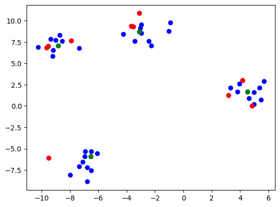
Plotting the found prototypes (green) and criticisms (red)
You’ll notice that I provided the option to use a separate kernel for prototype and criticism selection. This is because I’ve found that results for criticisms especially can be extremely sensitive to the sigma hyperparameter. This is an unfortunate limitation of the MMD Critic method and kernel methods in general. Overall, I’ve found good results using a large sigma for prototypes and a smaller one for criticisms.
We can also, of course, use a more complicated dataset. Here, for instance, is the method used on MNIST³:
from sklearn.datasets import fetch_openml
import numpy as np
from mmd_critic import MMDCritic
from mmd_critic.kernels import RBFKernel
# Load MNIST data
mnist = fetch_openml('mnist_784', version=1)
images = (mnist['data'].astype(np.float32)).to_numpy() / 255.0
labels = mnist['target'].astype(np.int64)
critic = MMDCritic(images[:15000], RBFKernel(2.5), RBFKernel(0.025))
protos, _ = critic.select_prototypes(40)
criticisms, _ = critic.select_criticisms(40, protos)
which gets us the following prototypes
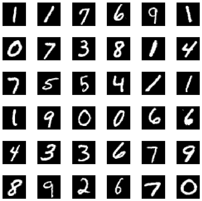
Prototypes found by MMD critic for MNIST. MNIST is free for commercial use under the GPL-3.0 License.
and criticisms
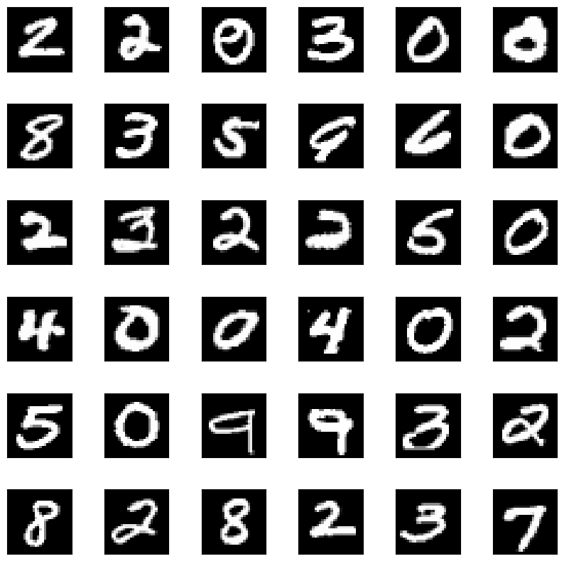
Criticisms found by the MMD Critic method
Pretty neat, huh?
Conclusions
And that’s about it for the MMD-Critic method. It is quite simple at the core, and it is nice to use save for having to fiddle with the Sigma hyperparameter. I hope that the newly released Python package gives it more use.
Please contact mchak@calpoly.edu for any inquiries. All images by author unless stated otherwise.
Footnotes
[1] You may be familiar with RKHSs and kernels if you’ve ever studied SVMs and the kernel trick — the kernels used there are just inner products in some RKHS. The most common is the RBF kernel, for which the associated RKHS of functions is an infinite-dimensional set of smooth functions.
[2] I have not read this source beyond a brief skim. It seems mostly irrelevant, and the log determinant regularizer is fairly simple to implement. If you want to read it though, go for it.
[3] For legal reasons, you can find a repository with the MNIST dataset here. It is free for commercial use under the GPL-3.0 License.
References
[1] https://onlinelibrary.wiley.com/doi/book/10.1002/9780470316801
[2]https://proceedings.neurips.cc/paper_files/paper/2016/file/5680522b8e2bb01943234bce7bf84534-Paper.pdf
[3] https://f0nzie.github.io/interpretable_ml-rsuite/proto.html#examples-5
[4] https://jmlr.csail.mit.edu/papers/volume13/gretton12a/gretton12a.pdf
[5] https://www.stat.cmu.edu/~ryantibs/journalclub/mmd.pdf
[6] https://jmlr.org/papers/volume9/krause08a/krause08a.pdf

The MMD-Critic Method, Explained was originally published in Towards Data Science on Medium, where people are continuing the conversation by highlighting and responding to this story.
Despite being a powerful tool for data summarization, the MMD-Critic method has a surprising lack of both usage and “coverage”. Perhaps this is because simpler and more established methods for data summarization exist (e.g. K-medoids, see [1] or, more simply, the Wikipedia page), or perhaps this is because no Python package for the method existed (before now). Regardless, the results presented in the original paper [2] warrant more use than MMD-Critic has currently. As such, I’ll explain the MMD-Critic method here with as much clarity as possible. I’ve also published an open-source Python package with an implementation of the technique so you can use it easily.
Prototypes and Criticisms
Before jumping into the MMD-Critic method itself, it’s worth discussing what exactly we’re trying to accomplish. Ultimately, we wish to take a dataset and find examples that are representative of the data (prototypes), as well as edge-case examples that may confound our machine learning models (criticisms).
Prototypes and criticisms for the MNIST dataset, taken from [2].
There are many reasons why this may be useful:
- We can get a very nice summarized view of our dataset by seeing both stereotypical and atypical examples
- We can test models on the criticisms to see how they handle edge cases (this is, for obvious reasons, very important)
- Though perhaps not as useful, we can use prototypes to create a naturally explainable K-means-esque algorithm wherein the closest prototype to the new data point is used to label it. Then explanations are simple since we just show the user the most similar data point.
- More
You can see section 6.3 in this book for more info on the applications of this (and for a decent explanation of MMD-Critic as well), but it suffices to say that finding these examples is useful for a wide variety of reasons. MMD-Critic allows us to do this.
Maximal Mean Discrepancy
I unfortunately cannot claim to have a hyper-rigorous understanding of Maximal Mean Discrepancy (MMD), as such an understanding would require a strong background in functional analysis. If you have such a background, you can find the paper that introduced the measure here.
In simple terms though, MMD is a way to determine the difference between two probability distributions. Formally, for two probability distributions P and Q, we define the MMD of the two as
The formula for the MMD of two distributions P, Q
Here, F is any function space — that is, any set of functions with the same domain and codomain. Note also that the notation x~P means that we are treating x as if it’s a random variable drawn from the distribution P — that is, x is described by P. This formula thus finds the highest difference in the expected values of X and Y when they are transformed by some function from our space F.
This may be a little hard to wrap your head around, but here’s an example. Suppose that X is Uniform(0, 1) (i.e. a distribution that is equivalent to picking a random number from 0 to 1), and Y is Uniform(-1, 1) . Let’s also let F be a fairly simple family containing three functions — f(x) = 0, f(x) = x, and f(x) = x². Iterating over each function in our space, we get:
- In the f(x) = 0 case, E[f(x)] when x ~ P is 0 since no matter what x we choose, f(x) will be 0. The same holds for when x ~ Q. Thus, we get a mean discrepancy of 0
- In the f(x) = x case, we have E[f(x)] = 0.5 for the P case and 0 for the Q case, so our mean discrepancy is 0.5
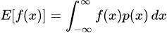
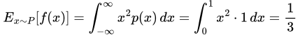
- In the f(x) = x² case, we note that
Formula for the expected value of a random variable x transformed by a function f
thus in the P case, we get
Expected value of f(x) under the distribution P
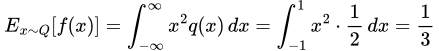
and in the Q case, we get
Expected value of f(x) under the distribution Q
thus our discrepancy in this case is also 0. The supremum over our function space is thus 0.5, so that’s our MMD.
You may now notice a few problems with our MMD. It seems highly dependent on our choice of function space and also appears highly expensive (or even impossible) to compute for a large or infinite function space. Not only that, but it also requires us to know our distributions P and Q, which is not realistic.
The latter problem is easily solvable, as we can rewrite our MMD metric to use estimates of P and Q based on our dataset:
MMD using estimates of P and Q
Here, our x’s are our samples from the dataset drawing from P, and the y’s are the samples drawn from Q.
The first two problems are solvable with a bit of extra math. Without going into too much detail, it turns out that if F is something called a Reproducing Kernel Hilbert Space (RKHS), we know what function is going to give us our MMD in advance. Namely, it’s the following function, called the witness function:
Our optimal f(x) in an RKHS
where k is the kernel (inner product) associated with the RKHS¹. Intuitively, this function “witnesses” the discrepancy between P and Q at the point x.
We thus only need to choose a sufficiently expressive RKHS/kernel — usually, the RBF kernel is used which has the kernel function
The RBF kernel, where sigma is a hyperparameter
This generally gets fairly intuitive results. Here, for instance, is the plot of the witness function with the RBF kernel when estimated (in the same way as mentioned before — that is, replacing expectations with a sum) on two datasets drawn from Uniform(-0.5, 0.5) and Uniform(-1, 1) :
Values of the witness function at different points for two uniform distributions
The code for generating the above graph is here:
import numpy as np
import matplotlib.pyplot as plt
import seaborn as sns
def rbf(v1, v2, sigma=0.5):
return np.exp(-(v2 - v1) ** 2/(2 * sigma**0.5))
def comp_wit_fn(x, d1, d2):
return 1/len(d1) * sum([rbf(x, dp) for dp in d1]) - 1/len(d2) * sum([rbf(x, dp) for dp in d2])
low1, high1 = -0.5, 0.5 # Range for the first uniform distribution
low2, high2 = -1, 1 # Range for the second uniform distribution
# Generate data for the uniform distributions
data1 = np.random.uniform(low1, high1, 10000)
data2 = np.random.uniform(low2, high2, 10000)
# Generate a range of x values for which to compute comp_wit_fn
x_values = np.linspace(min(low1 * 2, low2 * 2), max(high1 * 2, high2 * 2), 100)
comp_wit_values = [comp_wit_fn(x, data1, data2) for x in x_values]
sns.kdeplot(data1, label=f'Uniform({low1}, {high1})', color='blue', fill=True)
sns.kdeplot(data2, label=f'Uniform({low2}, {high2})', color='red', fill=True)
plt.plot(x_values, comp_wit_values, label='Witness Function', color='green')
plt.xlabel('Value')
plt.ylabel('Density / Wit Fn')
plt.legend()
plt.show()
The MMD-Critic Method, Finally
The idea behind MMD-Critic is now fairly simple — if we want to find k prototypes, we need to find the set of prototypes that best matches the distribution of the original dataset given by their squared MMD. In other words, we wish to find a subset P of cardinality k of our dataset that minimizes MMD²(F, X, P). Without going into too much detail about why, the square MMD is given by
The square MMD metric, with X ~ P, Y ~ Q, and k the kernel for our RKHS F
After finding these prototypes, we then select the points where the hypothetical distribution of our prototypes is most different from our dataset distribution as criticisms. As we’ve seen before, the difference between two distributions at a point can be measured by our witness function, so we just find points that maximize its absolute value in the context of X and P. In other words, we define our criticism “score” as
The “score” for a criticism c
Or, in the more usable approximate form,
The approximated S(c) for a criticism c
Then, to find our desired amount of criticisms, say m of them, we simply wish to find the set C of size m that maximizes
To promote picking more varied criticisms, the paper also suggests adding a regularizer term that encourages selected criticisms to be as far apart as possible. The suggested regularizer in the paper is the log determinant regularizer, though this is not required. I won’t go into much detail here since it’s not critical, but the paper suggests reading [6]².
We can thus implement an extremely naive MMD-Critic without criticism regularization as follows (do NOT use this):
import math
import itertools
def euc_distance(p1, p2):
return math.sqrt(sum((x - y) ** 2 for x, y in zip(p1, p2)))
def rbf(v1, v2, sigma=0.5):
return math.exp(-euc_distance(v1, v2) ** 2/(2 * sigma**0.5))
def mmd_sq(X, Y, sigma=0.5):
sm_xx = 0
for x in X:
for x2 in X:
sm_xx += rbf(x, x2, sigma)
sm_xy = 0
for x in X:
for y in Y:
sm_xy += rbf(x, y, sigma)
sm_yy = 0
for y in Y:
for y2 in Y:
sm_yy += rbf(y, y2, sigma)
return 1/(len(X) ** 2) * sm_xx \
- 2/(len(X) * len(Y)) * sm_xy \
+ 1/(len(Y) ** 2) * sm_yy
def select_protos(X, n, sigma=0.5):
min_score, min_sub = math.inf, None
for subset in itertools.combinations(X, n):
new_mmd = mmd_sq(X, subset, sigma)
if new_mmd < min_score:
min_score = new_mmd
min_sub = subset
return min_sub
def criticism_score(criticism, prototypes, X, sigma=0.5):
return abs(1/len(X) * sum([rbf(criticism, x, sigma) for x in X])\
- 1/len(prototypes) * sum([rbf(criticism, p, sigma) for p in prototypes]))
def select_criticisms(X, P, n, sigma=0.5):
candidates = [c for c in X if c not in P]
max_score, crits = -math.inf, []
for subset in itertools.combinations(candidates, n):
new_score = sum([criticism_score(c, P, X, sigma) for c in subset])
if new_score > max_score:
max_score = new_score
crits = subset
return crits
Optimizing MMD-Critic
The above implementation is so impractical that, when I ran it, I failed to find 5 prototypes in a dataset with 25 points in a reasonable time. This is because our MMD calculation is O(max(|X|, |Y|)²), and iterating over every length-n subset is O(C(|X|, n)) (where C is the choose function), which gives us a horrendous runtime complexity.
Disregarding using more efficient computation methods (e.g. using pure numpy/numexpr/matrix calculations instead of loops/whatever) and caching repeated calculations, there are a few optimizations we can make on the theoretical level. Firstly, the most obvious slowdown we have is looping over the C(|X|, n) subsets in our prototype and criticism methods. Instead of that, we can use an approximation that loops n times, greedily selecting the best prototype each time. This allows us to change our prototype selection code to
def select_protos(X, n, sigma=0.5):
protos = []
for _ in range
:min_score, min_proto = math.inf, None
for cand in X:
if cand in protos:
continue
new_score = mmd_sq(X, protos + [cand], sigma)
if new_score < min_score:
min_score = new_score
min_proto = cand
protos.append(min_proto)
return protos
and similar for the criticisms.
There’s one other important lemma that makes this problem much more optimizable. It turns out that by changing our prototype selection into a minimization problem and adding a regularization term to the cost, we can compute the cost function very efficiently with matrix operations. I won’t go into much detail here, but you can check out the original paper for details.
Playing With the MMD-Critic Package
Now that we understand the MMD-Critic method, we can finally play with it! You can install it by running
pip install mmd-critic
The implementation in the package itself is much faster than the one presented here, so don’t worry.
We can run a fairly simple example using blobs as such:
from sklearn.datasets import make_blobs
from mmd_critic import MMDCritic
from mmd_critic.kernels import RBFKernel
n_samples = 50 # Total number of samples
centers = 4 # Number of clusters
cluster_std = 1 # Standard deviation of the clusters
X, _ = make_blobs(n_samples=n_samples, centers=centers, cluster_std=cluster_std, n_features=2, random_state=42)
X = X.tolist()
# MMD critic with the kernel used for the prototypes being an RBF with sigma=1,
# for the criticisms one with sigma=0.025
critic = MMDCritic(X, RBFKernel(1), RBFKernel(0.025))
protos, _ = critic.select_prototypes(centers)
criticisms, _ = critic.select_criticisms(10, protos)
Then plotting the points and criticisms gets us
Plotting the found prototypes (green) and criticisms (red)
You’ll notice that I provided the option to use a separate kernel for prototype and criticism selection. This is because I’ve found that results for criticisms especially can be extremely sensitive to the sigma hyperparameter. This is an unfortunate limitation of the MMD Critic method and kernel methods in general. Overall, I’ve found good results using a large sigma for prototypes and a smaller one for criticisms.
We can also, of course, use a more complicated dataset. Here, for instance, is the method used on MNIST³:
from sklearn.datasets import fetch_openml
import numpy as np
from mmd_critic import MMDCritic
from mmd_critic.kernels import RBFKernel
# Load MNIST data
mnist = fetch_openml('mnist_784', version=1)
images = (mnist['data'].astype(np.float32)).to_numpy() / 255.0
labels = mnist['target'].astype(np.int64)
critic = MMDCritic(images[:15000], RBFKernel(2.5), RBFKernel(0.025))
protos, _ = critic.select_prototypes(40)
criticisms, _ = critic.select_criticisms(40, protos)
which gets us the following prototypes
Prototypes found by MMD critic for MNIST. MNIST is free for commercial use under the GPL-3.0 License.
and criticisms
Criticisms found by the MMD Critic method
Pretty neat, huh?
Conclusions
And that’s about it for the MMD-Critic method. It is quite simple at the core, and it is nice to use save for having to fiddle with the Sigma hyperparameter. I hope that the newly released Python package gives it more use.
Please contact mchak@calpoly.edu for any inquiries. All images by author unless stated otherwise.
Footnotes
[1] You may be familiar with RKHSs and kernels if you’ve ever studied SVMs and the kernel trick — the kernels used there are just inner products in some RKHS. The most common is the RBF kernel, for which the associated RKHS of functions is an infinite-dimensional set of smooth functions.
[2] I have not read this source beyond a brief skim. It seems mostly irrelevant, and the log determinant regularizer is fairly simple to implement. If you want to read it though, go for it.
[3] For legal reasons, you can find a repository with the MNIST dataset here. It is free for commercial use under the GPL-3.0 License.
References
[1] https://onlinelibrary.wiley.com/doi/book/10.1002/9780470316801
[2]https://proceedings.neurips.cc/paper_files/paper/2016/file/5680522b8e2bb01943234bce7bf84534-Paper.pdf
[3] https://f0nzie.github.io/interpretable_ml-rsuite/proto.html#examples-5
[4] https://jmlr.csail.mit.edu/papers/volume13/gretton12a/gretton12a.pdf
[5] https://www.stat.cmu.edu/~ryantibs/journalclub/mmd.pdf
[6] https://jmlr.org/papers/volume9/krause08a/krause08a.pdf
The MMD-Critic Method, Explained was originally published in Towards Data Science on Medium, where people are continuing the conversation by highlighting and responding to this story.