Training simulated humanoid robots to fight using five new Reinforcement Learning papers
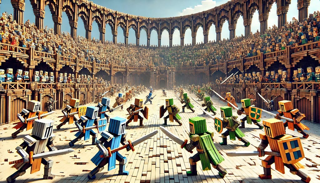
Generated with GPT-4
I remembered the old TV show Battlebots recently and wanted to put my own spin on it. So I trained simulated humanoid robots to fight using five new Reinforcement Learning papers.
By reading below, you’ll learn the theory and math of how these five Reinforcement Learning algorithms work, see me implement them, and see them go head to head to determine the champion!
Setting up the Simulation Environment:
I used the Unity machine learning agents simulator and built each robotic body with 21 actuators on 9 joints, 10 by 10 RGB vision through a virtual camera in their head, and a sword and shield. I then wrote the C# code defining their rewards and physics interactions. Agents can earn rewards in three main ways:
Agents get reset after 1000 timesteps, and I parallelized the environment massively for training.
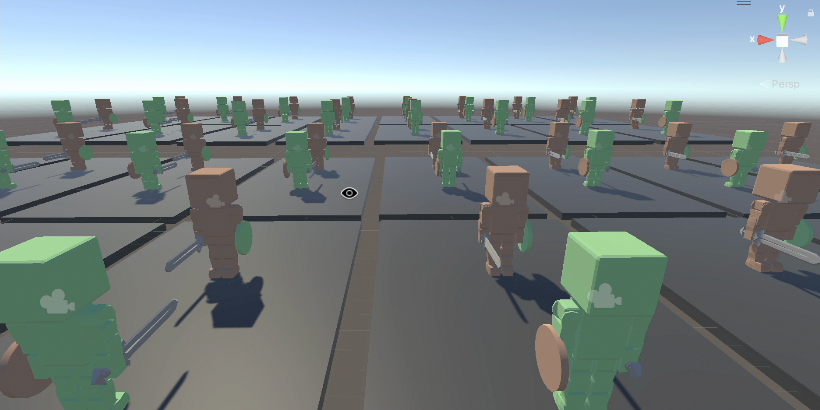
Massively parallelized training environment, my screenshot
Then it was time to write the algorithms. To understand the algorithms I used, it’s critical to understand what Q-Learning is, so let’s find out!
Q Learning (skip ahead if you’re familiar)
In Reinforcement Learning, we let an agent take actions to explore its environment, and reward it positively or negatively based on how close it is to the goal. How does the agent adjust its decision-making criteria to account for receiving better rewards?
Q Learning offers a solution. In Q Learning, we track Q-function Q(s,a), which tracks the expected return after action a_t from state s_t.
Q(s, a) = R(s, a) + γ * E[Q(s_t + 1, a_t + 1)] + γ² * E[Q(s_t + 2, a_t + 2) + …]
Where R(s,a) is the reward for the current state and action, y is the discount factor (a hyperparameter), and E[] is expected value.
If we properly learn this Q function, we can simply choose the action which returns the highest Q-value.
How do we learn this Q function?
Starting from the end of the episode, where we know the true Q value for certain (just our current reward), we can use recursion to fill in the previous Q values using the following update equation:
Q(s,a) ← (1 — α) Q(s,a) + α * [r + γ * max_a’ Q(s’,a’)]
Where α is the learning rate, r is the immediate reward, γ is the discount factor (weight parameter), s’ is the next state, and max_a’ Q(s’,a’) is the maximum Q-value for the next state over all possible actions
Essentially, our new Q value becomes old Q value plus small percentage of the difference between the current reward + the next largest Q value and the old Q value. Now, when our agent wants to choose an action, they can select the action which yields the greatest Q value (expected reward)
You might notice a potential issue though: we are evaluating the Q function on every possible action at every timestep. This is fine if we have a limited number of possible actions in a discrete space, but this paradigm breaks down in continuous actions spaces, where it is no longer possible to efficiently evaluate the Q function over the infinite number of possible actions. This brings us to our first competing algorithm: (DDPG)
Deep Deterministic Policy Gradient (DDPG)
DDPG tries to use Q Networks in continuous action spaces in a novel way.
Innovation 1: Actor and Critic
We can’t use the Q network to make our decisions directly, but we can use it to train another separate decision-making function. This is the actor-critic setup: the Actor is the policy decides actions, and the Critic determines future expected rewards based on these actions
Target Critic: Q_target(s,a) = r + γ * Q’(s’, μ’(s’))
Where r is the immediate reward, γ is the discount factor, s’ is the next state, μ’(s’) is the target policy network’s action for the next state, Q’ is the target critic network, Target Actor: Gradient of expected return wrt policy ≈ 1/N * Σ ∇a Q(s, a)|a=μ(s) * ∇θ_μ μ(s)
Essentially, over N samples, how does Q value of action chosen by policy (wrt policy changes, which change wrt policy params
To update both, we use a Stochastic Gradient Ascent update with lr * gradient on MSE loss of current Q and target Q. Note that both actor and critic are implemented as neural networks.
Innovation 2: Deterministic Action Policy
Our policy can either be deterministic (guaranteed action for each state) or stochastic (sample action for each state according to a probability distribution). The deterministic action policy for efficient evaluation of Q function (singular recursive evaluations since only one action for each state).
How do we explore with a deterministic policy, though? Won’t we be stuck running the same actions over and over again? This would be the case, however, we can increase the agent’s exploration by adding randomly generated noise to encourage exploration (a bit like how mutation benefits evolution by allowing it to explore unique genetic possibilities)
Innovation 3: Batch Learning in interactive environments
We also want to get more bang for our buck with each timestep observed (which consists of state action reward next state): so we can store previous tuples of timestep data and use it for training in the future
This allows us to use batch learning offline (which means using previously collected data instead of interaction through an environment), plus lets us parallelize to increase training speed with a GPU. We also now have independent identically distributed data as opposed to the biased sequential data we get regularly (where the value of a datapoint depends on previous datapoints)
Innovation 4: Target Networks
Usually Q Learning with NNs is too unstable and doesn’t converge to an optimal solution as easily because updates are too sensitive/powerful
Thus, we use target actor and critic networks, which interact with the environment and change to be partially but not fully closer to the real actor and critic during training ((large factor)target + (small factor)new)
Algorithm Runthrough and Code
Knights-of-Papers/src/DDPG/DDPG.py at main · AlmondGod/Knights-of-Papers
Soft Actor-Critic (SAC)
DDPG does have a few issues. Namely, Critic updates include bellman equation: Q(s,a) = r + max Q(s’a’), but NN as Q network approximators yield lot of noise, and max of noise means we overestimate, thus we become too optimistic about our policy and reward mediocre actions. Notoriously, DPPG also requires extensive hyperparameter tuning (including noise added) and doesn’t guarantee convergence to an optimal solution unless its hyperparameters are within a narrow range.
Innovation 1: Maximum Entropy Reinforcement Learning
Instead of the actor trying to purely maximize reward, the actor now maximizes reward + entropy:
Why use entropy?
Entropy is essentially how uncertain are we of a certain outcome (ex coin max entropy biased coined less entropy coin always heads has 0 entropy: show formula).
By including entropy as a maximization factor, we incentivize wide exploration and thus improves sensitivity to local optima, by allowing for more consistent and stable exploration of high dimensional spaces (why is this better than random noise). Alpha: param that weights how much to prioritize entropy, automatically tuned (how?)
Innovation 2: Two Q functions
This change aims to solve the Bellman overestimation bias of the Q function by training two Q networks independently and using the minimum of the two in policy improvement step,
Algorithm Runthrough and Code
Knights-of-Papers/src/SAC/SAC.py at main · AlmondGod/Knights-of-Papers
I2A with PPO
Two algorithms here (bonus alg layer works on top of any algorithm)
Proximal Policy Optimization (PPO)
Using a different approach to that of DDPG and SAC, our goal is a scalable, data-efficient, robust convergence algorithm (not sensitive to definition of hyperparameters.
Innovation 1: Surrogate Objective Function
The surrogate objective allows off-policy training so we can use a much wider variety of data (especially advantageous to real-world scenarios where vast pre-existing datasets exist).
Before we discuss surrogate objective, the concept of Advantage is critical to understand. Advantage is the:difference between expected reward at s after taking s and expected reward at s. Essentially, it quantifies to what degree an action a better or worse than the ‘average’ action.
We estimate it as A = Q(a,s) — V(a) where Q is action-value (expected return after action a) and V is state-value (expected return from current state), and both are learned
Now, the surrogate objective:
J(θ) = Ê_t [ r_t(θ) Â_t ]
Where:
This is equivalent to quantifying how well the new policy improves the likelihood of higher return actions and decreases likelihood of lower return actions.
Innovation 2: Clipped Objective Function
This is another way to solve the oversized policy update issue towards more stable learning.
L_CLIP(θ) = E[ min( r(θ) * A, clip(r(θ), 1-ε, 1+ε) * A ) ]
The clipped objective is minimum of the real surrogate and the surrogate where the ratio is clipped between 1 — epsilon and 1 + epsilon (basically trust region of unmodified ratio). Epsilon is usually ~0.1/0.2
It essentially chooses more conservative of clipped and normal ratio.
The actual PPO objective:
L^{PPO}(θ) = Ê_t [ L^{CLIP}(θ) — c_1 * L^{VF}(θ) + c_2 * Sπ_θ ]
Where:
Essentially we’re prioritizing higher entropy, lower value function, and higher clipped Advantage
PPO also uses minibatching and alternates data training.
Algorithm Runthrough and Code
Knights-of-Papers/src/I2A-PPO/gpuI2APPO.py at main · AlmondGod/Knights-of-Papers
Imagination-Augmented Agents
Our goal here is to create an extra embedding vector input to any other algorithm to give key valuable information and act as a ‘mental model’ of the environment
Innovation: Imagination Vector
The Imagination vector allows us to add an extra embedding vector to our agent’s observations to encode multiple ‘imagined future runs’ of actions and evaluations of their rewards (goal is to “see the future” and “think before acting”).
How do we calculate it? We use a learned environment approximation function, which tries to simulate the environment (this is called model-based learning because were attempting to learn a model of the environment). We pair this with a rollout policy, which is very simple and fast-executing policy (usually random) to decide on actions by which to “explore the future”. By running the environment approximator on the rollout policy, we can explore future actions and their rewars, then find a way to represent all these imagined future actions and rewards in one vector. A notable drawback to note: as you’d expect, it adds a lot of training and makes large amounts of data more necessary.
Combined I2A-PPO Algorithm Runthrough and Code
Decision Transformer
Our goal here is to use the advantage of transformer architecture for reinforcement learning. With Decision Transformer, we can identify important rewards among sparse/distracting rewards, enjoy a wider distribution modeling for greater generalization and knowledge transfer, and learn from pre-obtained suboptimal limited data (called offline learning).
For Decision Transformers, we essentially cast Reinforcement Learning as sequence modeling problem.
Innovation 1: Transformers
If you want to truly understand transformers, I recommend the karpathy building GP2 from scratch video. Here’s a quick Transformers review as it applies to DT:
We have sequences of tokens representing states, actions, returns to go (the sum of future rewards expected to be received), and timesteps. Our goal is now to take in a sequence of tokens and predict the next action: this will act as our policy.
These tokens all have keys, values, and queries that we combine using intricate networks to express relationships between each element. We then combine these relationships into an ‘embedding’ vector which encodes the relationships between the inputs. This process is known as Attention.
Note that a ‘causal self-attention mask’ ensures embeddings can only relate to embeddings that came before them in the sequence, so we can’t use the future to predict the future, use the past information to predict the future (since our goal is to predict next action).
Once we have this embedding vector, we pass it through neural network layers (the analogy Karpathy uses is that here, we ‘reason about relationships’ between the tokens).
These two combined (find relationships between tokens with Attention, reason about relationships with our NN layers) are one head of Transformers, which we stack on itself many times. At the end of these heads, we use a learned neural network layer to convert the output to our action space size and requirements.
By the way, at inference time, we predefine returns to go as our desired total reward at the end.
Algorithm Runthrough and Code
Knights-of-Papers/src/Decision-Transformer/DecisionTransformer.py at main · AlmondGod/Knights-of-Papers
Results
To train these models, I ran the algorithms on an NVIDIA RTX 4090 to take advantage of these algorithms GPU acceleration innovations. Thank you vast.ai! Here are the loss curves:
DDPG Loss (2000 Episodes)
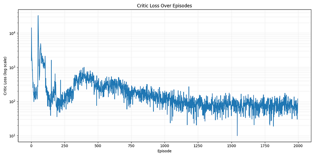
Matplotlib Loss Chart, me
I2APPO Loss (3500 Episodes)
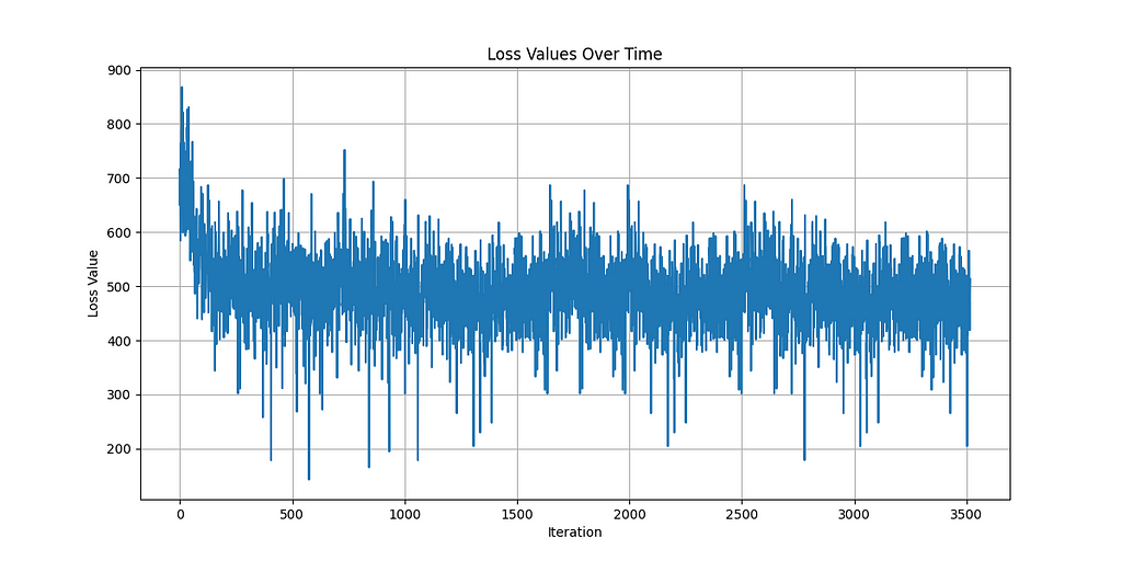
Matplotlib Loss Chart, me
SAC Loss (5000 Episodes)
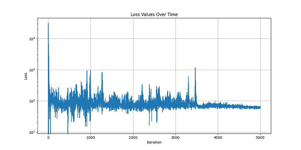
Matplotlib Loss Chart, me
Decision Transformer Loss (1600 Episodes, loss recorded every 40)
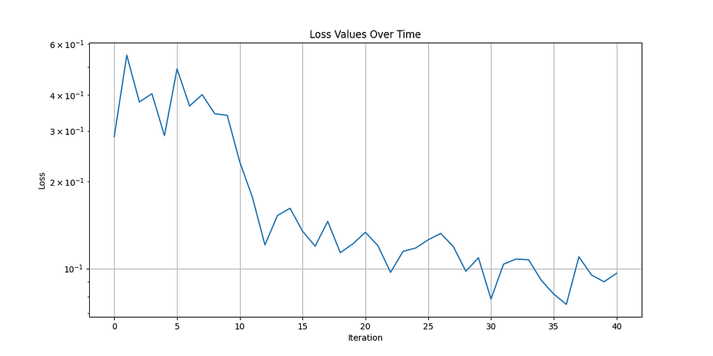
Matplotlib Loss Chart, me
By comparing the algorithms’ results (subjectively and weighted by time taken to train), I found Decision Transformer to perform the best! This makes sense considering DT is built specifically to take advantage of GPUs. Watch the video I made to see the algorithms’ actual performance. The models learned to crawl and stop falling over but still had a ways to go before they would be expert fighters.
Areas of Improvement:
I learned just how hard training a humanoid is. We’re operating in both a high-dimensional input space (both visual RGB and actuator positions/velocities) combined with an incredibly high-dimensional output space (27-dimensional continuous space).
From the beginning, the best I was hoping for was that they crawl to each other and touch swords, though even this was a challenge. Most of the training runs didn’t even get to experience the high reward of touching ones sword to the opponent, since walking alone was too hard.
The main dimension for improvement is simply increasing the time to train and amount of compute used. As we’ve seen in the modern AI revolution, these increased compute and data trends seem to have no upper limit!
Most importantly, I learned a lot! For next time, I would use NVIDIA’s skill embeddings or Lifelong Learning to allow the robots to learn to walk before they learn to fight!
To see the video I made walking through the process of creating this project, and see the robots fight, see this video below:
Thanks for making it to the end! Find me on Twitter @AlmondGodd if you’re interested in more!

The Tournament of Reinforcement Learning: DDPG, SAC, PPO, I2A, Decision Transformer was originally published in Towards Data Science on Medium, where people are continuing the conversation by highlighting and responding to this story.
Generated with GPT-4
I remembered the old TV show Battlebots recently and wanted to put my own spin on it. So I trained simulated humanoid robots to fight using five new Reinforcement Learning papers.
By reading below, you’ll learn the theory and math of how these five Reinforcement Learning algorithms work, see me implement them, and see them go head to head to determine the champion!
- Deep Deterministic Policy Gradient (DDPG)
- Decision Transformer
- Soft Actor-Critic (SAC)
- Imagination-Augmented Agents (I2A) with Proximal Policy Optimization (PPO)
Setting up the Simulation Environment:
I used the Unity machine learning agents simulator and built each robotic body with 21 actuators on 9 joints, 10 by 10 RGB vision through a virtual camera in their head, and a sword and shield. I then wrote the C# code defining their rewards and physics interactions. Agents can earn rewards in three main ways:
- Touching the sword to the opponent (‘Defeating’ their opponent)
- Keeping the y-position of their head above their body (to incentivize them to stand up)
- Going closer to their opponent than they were previously (to encourage agents to converge and fight)
Agents get reset after 1000 timesteps, and I parallelized the environment massively for training.
Massively parallelized training environment, my screenshot
Then it was time to write the algorithms. To understand the algorithms I used, it’s critical to understand what Q-Learning is, so let’s find out!
Q Learning (skip ahead if you’re familiar)
In Reinforcement Learning, we let an agent take actions to explore its environment, and reward it positively or negatively based on how close it is to the goal. How does the agent adjust its decision-making criteria to account for receiving better rewards?
Q Learning offers a solution. In Q Learning, we track Q-function Q(s,a), which tracks the expected return after action a_t from state s_t.
Q(s, a) = R(s, a) + γ * E[Q(s_t + 1, a_t + 1)] + γ² * E[Q(s_t + 2, a_t + 2) + …]
Where R(s,a) is the reward for the current state and action, y is the discount factor (a hyperparameter), and E[] is expected value.
If we properly learn this Q function, we can simply choose the action which returns the highest Q-value.
How do we learn this Q function?
Starting from the end of the episode, where we know the true Q value for certain (just our current reward), we can use recursion to fill in the previous Q values using the following update equation:
Q(s,a) ← (1 — α) Q(s,a) + α * [r + γ * max_a’ Q(s’,a’)]
Where α is the learning rate, r is the immediate reward, γ is the discount factor (weight parameter), s’ is the next state, and max_a’ Q(s’,a’) is the maximum Q-value for the next state over all possible actions
Essentially, our new Q value becomes old Q value plus small percentage of the difference between the current reward + the next largest Q value and the old Q value. Now, when our agent wants to choose an action, they can select the action which yields the greatest Q value (expected reward)
You might notice a potential issue though: we are evaluating the Q function on every possible action at every timestep. This is fine if we have a limited number of possible actions in a discrete space, but this paradigm breaks down in continuous actions spaces, where it is no longer possible to efficiently evaluate the Q function over the infinite number of possible actions. This brings us to our first competing algorithm: (DDPG)
Deep Deterministic Policy Gradient (DDPG)
DDPG tries to use Q Networks in continuous action spaces in a novel way.
Innovation 1: Actor and Critic
We can’t use the Q network to make our decisions directly, but we can use it to train another separate decision-making function. This is the actor-critic setup: the Actor is the policy decides actions, and the Critic determines future expected rewards based on these actions
Target Critic: Q_target(s,a) = r + γ * Q’(s’, μ’(s’))
Where r is the immediate reward, γ is the discount factor, s’ is the next state, μ’(s’) is the target policy network’s action for the next state, Q’ is the target critic network, Target Actor: Gradient of expected return wrt policy ≈ 1/N * Σ ∇a Q(s, a)|a=μ(s) * ∇θ_μ μ(s)
Essentially, over N samples, how does Q value of action chosen by policy (wrt policy changes, which change wrt policy params
To update both, we use a Stochastic Gradient Ascent update with lr * gradient on MSE loss of current Q and target Q. Note that both actor and critic are implemented as neural networks.
Innovation 2: Deterministic Action Policy
Our policy can either be deterministic (guaranteed action for each state) or stochastic (sample action for each state according to a probability distribution). The deterministic action policy for efficient evaluation of Q function (singular recursive evaluations since only one action for each state).
How do we explore with a deterministic policy, though? Won’t we be stuck running the same actions over and over again? This would be the case, however, we can increase the agent’s exploration by adding randomly generated noise to encourage exploration (a bit like how mutation benefits evolution by allowing it to explore unique genetic possibilities)
Innovation 3: Batch Learning in interactive environments
We also want to get more bang for our buck with each timestep observed (which consists of state action reward next state): so we can store previous tuples of timestep data and use it for training in the future
This allows us to use batch learning offline (which means using previously collected data instead of interaction through an environment), plus lets us parallelize to increase training speed with a GPU. We also now have independent identically distributed data as opposed to the biased sequential data we get regularly (where the value of a datapoint depends on previous datapoints)
Innovation 4: Target Networks
Usually Q Learning with NNs is too unstable and doesn’t converge to an optimal solution as easily because updates are too sensitive/powerful
Thus, we use target actor and critic networks, which interact with the environment and change to be partially but not fully closer to the real actor and critic during training ((large factor)target + (small factor)new)
Algorithm Runthrough and Code
- Initialize critic, actor, target critic and actor, replay buffer
- For the vision I use a CNN before any other layers (so the most important features of the vision are used by the algorithm)
- For each episode
- Observe state, select and execute action mu + noise
- Get reward, next state
- Store (s_t,a_t,r_t, s_(t+1)) in replay buffer
- sample rendom minibatch from buffer
- Update y_i = reward_i + gamma Q(s given theta)
- Evaluate recursively
- Update critic to minimize L = y_i — Q(s,a|theta)
- Update actor using policy gradient J expected recursive Q given policy
- Update targets to be large factor * targets + (1 — large factor) * actual
Knights-of-Papers/src/DDPG/DDPG.py at main · AlmondGod/Knights-of-Papers
Soft Actor-Critic (SAC)
DDPG does have a few issues. Namely, Critic updates include bellman equation: Q(s,a) = r + max Q(s’a’), but NN as Q network approximators yield lot of noise, and max of noise means we overestimate, thus we become too optimistic about our policy and reward mediocre actions. Notoriously, DPPG also requires extensive hyperparameter tuning (including noise added) and doesn’t guarantee convergence to an optimal solution unless its hyperparameters are within a narrow range.
Innovation 1: Maximum Entropy Reinforcement Learning
Instead of the actor trying to purely maximize reward, the actor now maximizes reward + entropy:
Why use entropy?
Entropy is essentially how uncertain are we of a certain outcome (ex coin max entropy biased coined less entropy coin always heads has 0 entropy: show formula).
By including entropy as a maximization factor, we incentivize wide exploration and thus improves sensitivity to local optima, by allowing for more consistent and stable exploration of high dimensional spaces (why is this better than random noise). Alpha: param that weights how much to prioritize entropy, automatically tuned (how?)
Innovation 2: Two Q functions
This change aims to solve the Bellman overestimation bias of the Q function by training two Q networks independently and using the minimum of the two in policy improvement step,
Algorithm Runthrough and Code
- Initialize actor, 2 Q functions, 2 target Q functions, replay buffer, alpha
- Repeat until convergence:
- For each environment step:
- Sample action from policy, observe next state and reward
- Store (s_t, a_t, r_t, s_t+1) in replay buffer
- For each update step:
- Sample batch
- Update Qs:
- Compute target y = reward plus minimum Q of policy + alpha entropy
- Minimize Q prediction — y
- Update policy to maximize Q of policy + alpha reward
- Update alpha to meet target entropy
- Update target Q networks (soft update targets to be large factor * targets + (1 — large factor) * actual)
Knights-of-Papers/src/SAC/SAC.py at main · AlmondGod/Knights-of-Papers
I2A with PPO
Two algorithms here (bonus alg layer works on top of any algorithm)
Proximal Policy Optimization (PPO)
Using a different approach to that of DDPG and SAC, our goal is a scalable, data-efficient, robust convergence algorithm (not sensitive to definition of hyperparameters.
Innovation 1: Surrogate Objective Function
The surrogate objective allows off-policy training so we can use a much wider variety of data (especially advantageous to real-world scenarios where vast pre-existing datasets exist).
Before we discuss surrogate objective, the concept of Advantage is critical to understand. Advantage is the:difference between expected reward at s after taking s and expected reward at s. Essentially, it quantifies to what degree an action a better or worse than the ‘average’ action.
We estimate it as A = Q(a,s) — V(a) where Q is action-value (expected return after action a) and V is state-value (expected return from current state), and both are learned
Now, the surrogate objective:
J(θ) = Ê_t [ r_t(θ) Â_t ]
Where:
- J(θ) is the surrogate objective
- Ê_t […] denotes the empirical average over a finite batch of samples
- r_t(θ) = π_θ(a_t|s_t) / π_θ_old(a_t|s_t) is likelihood of action in new policy / likelihood in old policy
- Â_t is the estimated advantage at timestep t
This is equivalent to quantifying how well the new policy improves the likelihood of higher return actions and decreases likelihood of lower return actions.
Innovation 2: Clipped Objective Function
This is another way to solve the oversized policy update issue towards more stable learning.
L_CLIP(θ) = E[ min( r(θ) * A, clip(r(θ), 1-ε, 1+ε) * A ) ]
The clipped objective is minimum of the real surrogate and the surrogate where the ratio is clipped between 1 — epsilon and 1 + epsilon (basically trust region of unmodified ratio). Epsilon is usually ~0.1/0.2
It essentially chooses more conservative of clipped and normal ratio.
The actual PPO objective:
L^{PPO}(θ) = Ê_t [ L^{CLIP}(θ) — c_1 * L^{VF}(θ) + c_2 * Sπ_θ ]
Where:
- L^{VF}(θ) = (V_θ(s_t) — V^{target}_t)²
- Sπ_θ is the entropy of the policy π_θ for state s_t
Essentially we’re prioritizing higher entropy, lower value function, and higher clipped Advantage
PPO also uses minibatching and alternates data training.
Algorithm Runthrough and Code
- For each iteration
- For each of N actors
- Run policy for T timesteps
- Compute advantages
- Optimize surrogate function with respect to policy for K epochs and minibatch size M < NT
- Update policy
Knights-of-Papers/src/I2A-PPO/gpuI2APPO.py at main · AlmondGod/Knights-of-Papers
Imagination-Augmented Agents
Our goal here is to create an extra embedding vector input to any other algorithm to give key valuable information and act as a ‘mental model’ of the environment
Innovation: Imagination Vector
The Imagination vector allows us to add an extra embedding vector to our agent’s observations to encode multiple ‘imagined future runs’ of actions and evaluations of their rewards (goal is to “see the future” and “think before acting”).
How do we calculate it? We use a learned environment approximation function, which tries to simulate the environment (this is called model-based learning because were attempting to learn a model of the environment). We pair this with a rollout policy, which is very simple and fast-executing policy (usually random) to decide on actions by which to “explore the future”. By running the environment approximator on the rollout policy, we can explore future actions and their rewars, then find a way to represent all these imagined future actions and rewards in one vector. A notable drawback to note: as you’d expect, it adds a lot of training and makes large amounts of data more necessary.
Combined I2A-PPO Algorithm Runthrough and Code
- Every time we collect observations for PPO:
- Initialize environment model and rollout pollicy
- For multiple ‘imagined runs’:
- run environment model starting from current state and deciding with rollout policy until a horizon to yield an imagination trajectory (s, a, r sequence)
- Imagination encoder: turns multiple of these imagined trajectories into a single input embedding for the actual decision making network
Decision Transformer
Our goal here is to use the advantage of transformer architecture for reinforcement learning. With Decision Transformer, we can identify important rewards among sparse/distracting rewards, enjoy a wider distribution modeling for greater generalization and knowledge transfer, and learn from pre-obtained suboptimal limited data (called offline learning).
For Decision Transformers, we essentially cast Reinforcement Learning as sequence modeling problem.
Innovation 1: Transformers
If you want to truly understand transformers, I recommend the karpathy building GP2 from scratch video. Here’s a quick Transformers review as it applies to DT:
We have sequences of tokens representing states, actions, returns to go (the sum of future rewards expected to be received), and timesteps. Our goal is now to take in a sequence of tokens and predict the next action: this will act as our policy.
These tokens all have keys, values, and queries that we combine using intricate networks to express relationships between each element. We then combine these relationships into an ‘embedding’ vector which encodes the relationships between the inputs. This process is known as Attention.
Note that a ‘causal self-attention mask’ ensures embeddings can only relate to embeddings that came before them in the sequence, so we can’t use the future to predict the future, use the past information to predict the future (since our goal is to predict next action).
Once we have this embedding vector, we pass it through neural network layers (the analogy Karpathy uses is that here, we ‘reason about relationships’ between the tokens).
These two combined (find relationships between tokens with Attention, reason about relationships with our NN layers) are one head of Transformers, which we stack on itself many times. At the end of these heads, we use a learned neural network layer to convert the output to our action space size and requirements.
By the way, at inference time, we predefine returns to go as our desired total reward at the end.
Algorithm Runthrough and Code
- For (R,s,a,t) in dataloader
- Predict action
- Model converts obs, vision (with convnet layer), rtg, and timestep to unique embeddings and adds timestep embedding to the others
- All three used as input to the transformer layers, at the end use action embedding
- compute MSEloss (a_pred-a)**2
- Perform SGD on the decision transformer model with the gradient of params wrt this loss
Knights-of-Papers/src/Decision-Transformer/DecisionTransformer.py at main · AlmondGod/Knights-of-Papers
Results
To train these models, I ran the algorithms on an NVIDIA RTX 4090 to take advantage of these algorithms GPU acceleration innovations. Thank you vast.ai! Here are the loss curves:
DDPG Loss (2000 Episodes)
Matplotlib Loss Chart, me
I2APPO Loss (3500 Episodes)
Matplotlib Loss Chart, me
SAC Loss (5000 Episodes)
Matplotlib Loss Chart, me
Decision Transformer Loss (1600 Episodes, loss recorded every 40)
Matplotlib Loss Chart, me
By comparing the algorithms’ results (subjectively and weighted by time taken to train), I found Decision Transformer to perform the best! This makes sense considering DT is built specifically to take advantage of GPUs. Watch the video I made to see the algorithms’ actual performance. The models learned to crawl and stop falling over but still had a ways to go before they would be expert fighters.
Areas of Improvement:
I learned just how hard training a humanoid is. We’re operating in both a high-dimensional input space (both visual RGB and actuator positions/velocities) combined with an incredibly high-dimensional output space (27-dimensional continuous space).
From the beginning, the best I was hoping for was that they crawl to each other and touch swords, though even this was a challenge. Most of the training runs didn’t even get to experience the high reward of touching ones sword to the opponent, since walking alone was too hard.
The main dimension for improvement is simply increasing the time to train and amount of compute used. As we’ve seen in the modern AI revolution, these increased compute and data trends seem to have no upper limit!
Most importantly, I learned a lot! For next time, I would use NVIDIA’s skill embeddings or Lifelong Learning to allow the robots to learn to walk before they learn to fight!
To see the video I made walking through the process of creating this project, and see the robots fight, see this video below:
Thanks for making it to the end! Find me on Twitter @AlmondGodd if you’re interested in more!
The Tournament of Reinforcement Learning: DDPG, SAC, PPO, I2A, Decision Transformer was originally published in Towards Data Science on Medium, where people are continuing the conversation by highlighting and responding to this story.