Part 3 of our Gaussian Splatting tutorial, showing how to render splats onto a 2D image
Finally, we reach the most intriguing phase of the Gaussian splatting process: rendering! This step is arguably the most crucial, as it determines the realism of our model. Yet, it might also be the simplest. In part 1 and part 2 of our series we demonstrated how to transform raw splats into a format ready for rendering, but now we actually have to do the work and render onto a fixed set of pixels. The authors have developed a fast rendering engine using CUDA, which can be somewhat challenging to follow. Therefore, I believe it is beneficial to first walk through the code in Python, using straightforward for loops for clarity. For those eager to dive deeper, all the necessary code is available on our GitHub.
Let’s discuss how to render each individual pixel. From our previous article, we have all the necessary components: 2D points, associated colors, covariance, sorted depth order, inverse covariance in 2D, minimum and maximum x and y values for each splat, and associated opacity. With these components, we can render any pixel. Given specific pixel coordinates, we iterate through all splats until we reach a saturation threshold, following the splat depth order relative to the camera plane (projected to the camera plane and then sorted by depth). For each splat, we first check if the pixel coordinate is within the bounds defined by the minimum and maximum x and y values. This check determines if we should continue rendering or ignore the splat for these coordinates. Next, we compute the Gaussian splat strength at the pixel coordinate using the splat mean, splat covariance, and pixel coordinates.
def compute_gaussian_weight(
pixel_coord: torch.Tensor, # (1, 2) tensor
point_mean: torch.Tensor,
inverse_covariance: torch.Tensor,
) -> torch.Tensor:
difference = point_mean - pixel_coord
power = -0.5 * difference @ inverse_covariance @ difference.T
return torch.exp(power).item()
We multiply this weight by the splat’s opacity to obtain a parameter called alpha. Before adding this new value to the pixel, we need to check if we have exceeded our saturation threshold. We do not want a splat behind other splats to affect the pixel coloring and use computing resources if the pixel is already saturated. Thus, we use a threshold that allows us to stop rendering once it is exceeded. In practice, we start our saturation threshold at 1 and then multiply it by min(0.99, (1 — alpha)) to get a new value. If this value is less than our threshold (0.0001), we stop rendering that pixel and consider it complete. If not, we add the colors weighted by the saturation * (1 — alpha) value and update the saturation as new_saturation = old_saturation * (1 — alpha). Finally, we loop over every pixel (or every 16x16 tile in practice) and render. The complete code is shown below.
def render_pixel(
self,
pixel_coords: torch.Tensor,
points_in_tile_mean: torch.Tensor,
colors: torch.Tensor,
opacities: torch.Tensor,
inverse_covariance: torch.Tensor,
min_weight: float = 0.000001,
) -> torch.Tensor:
total_weight = torch.ones(1).to(points_in_tile_mean.device)
pixel_color = torch.zeros((1, 1, 3)).to(points_in_tile_mean.device)
for point_idx in range(points_in_tile_mean.shape[0]):
point = points_in_tile_mean[point_idx, :].view(1, 2)
weight = compute_gaussian_weight(
pixel_coord=pixel_coords,
point_mean=point,
inverse_covariance=inverse_covariance[point_idx],
)
alpha = weight * torch.sigmoid(opacities[point_idx])
test_weight = total_weight * (1 - alpha)
if test_weight < min_weight:
return pixel_color
pixel_color += total_weight * alpha * colors[point_idx]
total_weight = test_weight
# in case we never reach saturation
return pixel_color
Now that we can render a pixel we can render a patch of an image, or what the authors refer to as a tile!
def render_tile(
self,
x_min: int,
y_min: int,
points_in_tile_mean: torch.Tensor,
colors: torch.Tensor,
opacities: torch.Tensor,
inverse_covariance: torch.Tensor,
tile_size: int = 16,
) -> torch.Tensor:
"""Points in tile should be arranged in order of depth"""
tile = torch.zeros((tile_size, tile_size, 3))
# iterate by tiles for more efficient processing
for pixel_x in range(x_min, x_min + tile_size):
for pixel_y in range(y_min, y_min + tile_size):
tile[pixel_x % tile_size, pixel_y % tile_size] = self.render_pixel(
pixel_coords=torch.Tensor([pixel_x, pixel_y])
.view(1, 2)
.to(points_in_tile_mean.device),
points_in_tile_mean=points_in_tile_mean,
colors=colors,
opacities=opacities,
inverse_covariance=inverse_covariance,
)
return tile
And finally we can use all of those tiles to render an entire image. Note how we check to make sure the splat will actually affect the current tile (x_in_tile and y_in_tile code).
def render_image(self, image_idx: int, tile_size: int = 16) -> torch.Tensor:
"""For each tile have to check if the point is in the tile"""
preprocessed_scene = self.preprocess(image_idx)
height = self.images[image_idx].height
width = self.images[image_idx].width
image = torch.zeros((width, height, 3))
for x_min in tqdm(range(0, width, tile_size)):
x_in_tile = (x_min >= preprocessed_scene.min_x) & (
x_min + tile_size <= preprocessed_scene.max_x
)
if x_in_tile.sum() == 0:
continue
for y_min in range(0, height, tile_size):
y_in_tile = (y_min >= preprocessed_scene.min_y) & (
y_min + tile_size <= preprocessed_scene.max_y
)
points_in_tile = x_in_tile & y_in_tile
if points_in_tile.sum() == 0:
continue
points_in_tile_mean = preprocessed_scene.points[points_in_tile]
colors_in_tile = preprocessed_scene.colors[points_in_tile]
opacities_in_tile = preprocessed_scene.sigmoid_opacity[points_in_tile]
inverse_covariance_in_tile = preprocessed_scene.inverse_covariance_2d[
points_in_tile
]
image[x_min : x_min + tile_size, y_min : y_min + tile_size] = (
self.render_tile(
x_min=x_min,
y_min=y_min,
points_in_tile_mean=points_in_tile_mean,
colors=colors_in_tile,
opacities=opacities_in_tile,
inverse_covariance=inverse_covariance_in_tile,
tile_size=tile_size,
)
)
return image
At long last now that we have all the necessary components we can render an image. We take all the 3D points from the treehill dataset and initialize them as gaussian splats. In order to avoid a costly nearest neighbor search we initialize all scale variables as .01 (Note that with such a small variance we will need a strong concentration of splats in one spot to be visible. Larger variance makes the process quite slow.). Then all we have to do is call render_image with the image number we are trying to emulate and as you an see we get a sparse set of point clouds that resemble our image! (Check out our bonus section at the bottom for an equivalent CUDA kernel using pyTorch’s nifty tool that compiles CUDA code!)
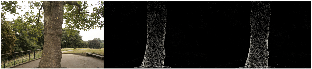
Actual image, CPU implementation, CUDA implementation. Image by author.
While the backwards pass is not part of this tutorial, one note should be made that while we start with only these few points, we soon have hundreds of thousands of splats for most scenes. This is caused by the breaking up of large splats (as defined by larger variance on axes) into smaller splats and removing splats that have extremely low opacity. For instance, if we truly initialized the scale to the mean of the three closest nearest neighbors we would have a majority of the space covered. In order to get fine detail we would need to break these down into much smaller splats that are able to capture fine detail. They also need to populate areas with very few gaussians. They refer to these two scenarios as over reconstruction and under reconstruction and define both scenarios by large gradient values for various splats. They then split or clone the splats depending on size (see image below) and continue the optimization process.
Although the backward pass is not covered in this tutorial, it’s important to note that we start with only a few points but soon have hundreds of thousands of splats in most scenes. This increase is due to the splitting of large splats (with larger variances on axes) into smaller ones and the removal of splats with very low opacity. For instance, if we initially set the scale to the mean of the three nearest neighbors, most of the space would be covered. To achieve fine detail, we need to break these large splats into much smaller ones. Additionally, areas with very few Gaussians need to be populated. These scenarios are referred to as over-reconstruction and under-reconstruction, characterized by large gradient values for various splats. Depending on their size, splats are split or cloned (see image below), and the optimization process continues.
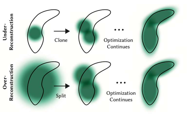
From the Author’s original paper on how gaussians are split or cloned in training. Source: https://arxiv.org/abs/2308.04079
And that is an easy introduction to Gaussian Splatting! You should now have a good intuition on what exactly is going on in the forward pass of a gaussian scene render. While a bit daunting and not exactly neural networks, all it takes is a bit of linear algebra and we can render 3D geometry in 2D!
Feel free to leave comments about confusing topics or if I got something wrong and you can always connect with me on LinkedIn or twitter!
Bonus — CUDA Code
Use PyTorch’s CUDA compiler to write a custom CUDA kernel!
def load_cuda(cuda_src, cpp_src, funcs, opt=True, verbose=False):
return load_inline(
name="inline_ext",
cpp_sources=[cpp_src],
cuda_sources=[cuda_src],
functions=funcs,
extra_cuda_cflags=["-O1"] if opt else [],
verbose=verbose,
)
class GaussianScene(nn.Module):
# OTHER CODE NOT SHOWN
def compile_cuda_ext(
self,
) -> torch.jit.ScriptModule:
cpp_src = """
torch::Tensor render_image(
int image_height,
int image_width,
int tile_size,
torch::Tensor point_means,
torch::Tensor point_colors,
torch::Tensor inverse_covariance_2d,
torch::Tensor min_x,
torch::Tensor max_x,
torch::Tensor min_y,
torch::Tensor max_y,
torch::Tensor opacity);
"""
cuda_src = Path("splat/c/render.cu").read_text()
return load_cuda(cuda_src, cpp_src, ["render_image"], opt=True, verbose=True)
def render_image_cuda(self, image_idx: int, tile_size: int = 16) -> torch.Tensor:
preprocessed_scene = self.preprocess(image_idx)
height = self.images[image_idx].height
width = self.images[image_idx].width
ext = self.compile_cuda_ext()
now = time.time()
image = ext.render_image(
height,
width,
tile_size,
preprocessed_scene.points.contiguous(),
preprocessed_scene.colors.contiguous(),
preprocessed_scene.inverse_covariance_2d.contiguous(),
preprocessed_scene.min_x.contiguous(),
preprocessed_scene.max_x.contiguous(),
preprocessed_scene.min_y.contiguous(),
preprocessed_scene.max_y.contiguous(),
preprocessed_scene.sigmoid_opacity.contiguous(),
)
torch.cuda.synchronize()
print("Operation took seconds: ", time.time() - now)
return image
#include <cstdio>
#include <cmath> // Include this header for expf function
#include <torch/extension.h>
__device__ float compute_pixel_strength(
int pixel_x,
int pixel_y,
int point_x,
int point_y,
float inverse_covariance_a,
float inverse_covariance_b,
float inverse_covariance_c)
{
// Compute the distance between the pixel and the point
float dx = pixel_x - point_x;
float dy = pixel_y - point_y;
float power = dx * inverse_covariance_a * dx + 2 * dx * dy * inverse_covariance_b + dy * dy * inverse_covariance_c;
return expf(-0.5f * power);
}
__global__ void render_tile(
int image_height,
int image_width,
int tile_size,
int num_points,
float *point_means,
float *point_colors,
float *image,
float *inverse_covariance_2d,
float *min_x,
float *max_x,
float *min_y,
float *max_y,
float *opacity)
{
// Calculate the pixel's position in the image
int pixel_x = blockIdx.x * tile_size + threadIdx.x;
int pixel_y = blockIdx.y * tile_size + threadIdx.y;
// Ensure the pixel is within the image bounds
if (pixel_x >= image_width || pixel_y >= image_height)
{
return;
}
float total_weight = 1.0f;
float3 color = {0.0f, 0.0f, 0.0f};
for (int i = 0; i < num_points; i++)
{
float point_x = point_means[i * 2];
float point_y = point_means[i * 2 + 1];
// checks to make sure we are within the bounding box
bool x_check = pixel_x >= min_x && pixel_x <= max_x;
bool y_check = pixel_y >= min_y && pixel_y <= max_y;
if (!x_check || !y_check)
{
continue;
}
float strength = compute_pixel_strength(
pixel_x,
pixel_y,
point_x,
point_y,
inverse_covariance_2d[i * 4],
inverse_covariance_2d[i * 4 + 1],
inverse_covariance_2d[i * 4 + 3]);
float initial_alpha = opacity * strength;
float alpha = min(.99f, initial_alpha);
float test_weight = total_weight * (1 - alpha);
if (test_weight < 0.001f)
{
break;
}
color.x += total_weight * alpha * point_colors[i * 3];
color.y += total_weight * alpha * point_colors[i * 3 + 1];
color.z += total_weight * alpha * point_colors[i * 3 + 2];
total_weight = test_weight;
}
image[(pixel_y * image_width + pixel_x) * 3] = color.x;
image[(pixel_y * image_width + pixel_x) * 3 + 1] = color.y;
image[(pixel_y * image_width + pixel_x) * 3 + 2] = color.z;
}
torch::Tensor render_image(
int image_height,
int image_width,
int tile_size,
torch::Tensor point_means,
torch::Tensor point_colors,
torch::Tensor inverse_covariance_2d,
torch::Tensor min_x,
torch::Tensor max_x,
torch::Tensor min_y,
torch::Tensor max_y,
torch::Tensor opacity)
{
// Ensure the input tensors are on the same device
torch::TensorArg point_means_t{point_means, "point_means", 1},
point_colors_t{point_colors, "point_colors", 2},
inverse_covariance_2d_t{inverse_covariance_2d, "inverse_covariance_2d", 3},
min_x_t{min_x, "min_x", 4},
max_x_t{max_x, "max_x", 5},
min_y_t{min_y, "min_y", 6},
max_y_t{max_y, "max_y", 7},
opacity_t{opacity, "opacity", 8};
torch::checkAllSameGPU("render_image", {point_means_t, point_colors_t, inverse_covariance_2d_t, min_x_t, max_x_t, min_y_t, max_y_t, opacity_t});
// Create an output tensor for the image
torch::Tensor image = torch::zeros({image_height, image_width, 3}, point_means.options());
// Calculate the number of tiles in the image
int num_tiles_x = (image_width + tile_size - 1) / tile_size;
int num_tiles_y = (image_height + tile_size - 1) / tile_size;
// Launch a CUDA kernel to render the image
dim3 block(tile_size, tile_size);
dim3 grid(num_tiles_x, num_tiles_y);
render_tile<<<grid, block>>>(
image_height,
image_width,
tile_size,
point_means.size(0),
point_means.data_ptr<float>(),
point_colors.data_ptr<float>(),
image.data_ptr<float>(),
inverse_covariance_2d.data_ptr<float>(),
min_x.data_ptr<float>(),
max_x.data_ptr<float>(),
min_y.data_ptr<float>(),
max_y.data_ptr<float>(),
opacity.data_ptr<float>());
return image;
}

A Python Engineer’s Introduction to 3D Gaussian Splatting (Part 3) was originally published in Towards Data Science on Medium, where people are continuing the conversation by highlighting and responding to this story.
Finally, we reach the most intriguing phase of the Gaussian splatting process: rendering! This step is arguably the most crucial, as it determines the realism of our model. Yet, it might also be the simplest. In part 1 and part 2 of our series we demonstrated how to transform raw splats into a format ready for rendering, but now we actually have to do the work and render onto a fixed set of pixels. The authors have developed a fast rendering engine using CUDA, which can be somewhat challenging to follow. Therefore, I believe it is beneficial to first walk through the code in Python, using straightforward for loops for clarity. For those eager to dive deeper, all the necessary code is available on our GitHub.
Let’s discuss how to render each individual pixel. From our previous article, we have all the necessary components: 2D points, associated colors, covariance, sorted depth order, inverse covariance in 2D, minimum and maximum x and y values for each splat, and associated opacity. With these components, we can render any pixel. Given specific pixel coordinates, we iterate through all splats until we reach a saturation threshold, following the splat depth order relative to the camera plane (projected to the camera plane and then sorted by depth). For each splat, we first check if the pixel coordinate is within the bounds defined by the minimum and maximum x and y values. This check determines if we should continue rendering or ignore the splat for these coordinates. Next, we compute the Gaussian splat strength at the pixel coordinate using the splat mean, splat covariance, and pixel coordinates.
def compute_gaussian_weight(
pixel_coord: torch.Tensor, # (1, 2) tensor
point_mean: torch.Tensor,
inverse_covariance: torch.Tensor,
) -> torch.Tensor:
difference = point_mean - pixel_coord
power = -0.5 * difference @ inverse_covariance @ difference.T
return torch.exp(power).item()
We multiply this weight by the splat’s opacity to obtain a parameter called alpha. Before adding this new value to the pixel, we need to check if we have exceeded our saturation threshold. We do not want a splat behind other splats to affect the pixel coloring and use computing resources if the pixel is already saturated. Thus, we use a threshold that allows us to stop rendering once it is exceeded. In practice, we start our saturation threshold at 1 and then multiply it by min(0.99, (1 — alpha)) to get a new value. If this value is less than our threshold (0.0001), we stop rendering that pixel and consider it complete. If not, we add the colors weighted by the saturation * (1 — alpha) value and update the saturation as new_saturation = old_saturation * (1 — alpha). Finally, we loop over every pixel (or every 16x16 tile in practice) and render. The complete code is shown below.
def render_pixel(
self,
pixel_coords: torch.Tensor,
points_in_tile_mean: torch.Tensor,
colors: torch.Tensor,
opacities: torch.Tensor,
inverse_covariance: torch.Tensor,
min_weight: float = 0.000001,
) -> torch.Tensor:
total_weight = torch.ones(1).to(points_in_tile_mean.device)
pixel_color = torch.zeros((1, 1, 3)).to(points_in_tile_mean.device)
for point_idx in range(points_in_tile_mean.shape[0]):
point = points_in_tile_mean[point_idx, :].view(1, 2)
weight = compute_gaussian_weight(
pixel_coord=pixel_coords,
point_mean=point,
inverse_covariance=inverse_covariance[point_idx],
)
alpha = weight * torch.sigmoid(opacities[point_idx])
test_weight = total_weight * (1 - alpha)
if test_weight < min_weight:
return pixel_color
pixel_color += total_weight * alpha * colors[point_idx]
total_weight = test_weight
# in case we never reach saturation
return pixel_color
Now that we can render a pixel we can render a patch of an image, or what the authors refer to as a tile!
def render_tile(
self,
x_min: int,
y_min: int,
points_in_tile_mean: torch.Tensor,
colors: torch.Tensor,
opacities: torch.Tensor,
inverse_covariance: torch.Tensor,
tile_size: int = 16,
) -> torch.Tensor:
"""Points in tile should be arranged in order of depth"""
tile = torch.zeros((tile_size, tile_size, 3))
# iterate by tiles for more efficient processing
for pixel_x in range(x_min, x_min + tile_size):
for pixel_y in range(y_min, y_min + tile_size):
tile[pixel_x % tile_size, pixel_y % tile_size] = self.render_pixel(
pixel_coords=torch.Tensor([pixel_x, pixel_y])
.view(1, 2)
.to(points_in_tile_mean.device),
points_in_tile_mean=points_in_tile_mean,
colors=colors,
opacities=opacities,
inverse_covariance=inverse_covariance,
)
return tile
And finally we can use all of those tiles to render an entire image. Note how we check to make sure the splat will actually affect the current tile (x_in_tile and y_in_tile code).
def render_image(self, image_idx: int, tile_size: int = 16) -> torch.Tensor:
"""For each tile have to check if the point is in the tile"""
preprocessed_scene = self.preprocess(image_idx)
height = self.images[image_idx].height
width = self.images[image_idx].width
image = torch.zeros((width, height, 3))
for x_min in tqdm(range(0, width, tile_size)):
x_in_tile = (x_min >= preprocessed_scene.min_x) & (
x_min + tile_size <= preprocessed_scene.max_x
)
if x_in_tile.sum() == 0:
continue
for y_min in range(0, height, tile_size):
y_in_tile = (y_min >= preprocessed_scene.min_y) & (
y_min + tile_size <= preprocessed_scene.max_y
)
points_in_tile = x_in_tile & y_in_tile
if points_in_tile.sum() == 0:
continue
points_in_tile_mean = preprocessed_scene.points[points_in_tile]
colors_in_tile = preprocessed_scene.colors[points_in_tile]
opacities_in_tile = preprocessed_scene.sigmoid_opacity[points_in_tile]
inverse_covariance_in_tile = preprocessed_scene.inverse_covariance_2d[
points_in_tile
]
image[x_min : x_min + tile_size, y_min : y_min + tile_size] = (
self.render_tile(
x_min=x_min,
y_min=y_min,
points_in_tile_mean=points_in_tile_mean,
colors=colors_in_tile,
opacities=opacities_in_tile,
inverse_covariance=inverse_covariance_in_tile,
tile_size=tile_size,
)
)
return image
At long last now that we have all the necessary components we can render an image. We take all the 3D points from the treehill dataset and initialize them as gaussian splats. In order to avoid a costly nearest neighbor search we initialize all scale variables as .01 (Note that with such a small variance we will need a strong concentration of splats in one spot to be visible. Larger variance makes the process quite slow.). Then all we have to do is call render_image with the image number we are trying to emulate and as you an see we get a sparse set of point clouds that resemble our image! (Check out our bonus section at the bottom for an equivalent CUDA kernel using pyTorch’s nifty tool that compiles CUDA code!)
Actual image, CPU implementation, CUDA implementation. Image by author.
While the backwards pass is not part of this tutorial, one note should be made that while we start with only these few points, we soon have hundreds of thousands of splats for most scenes. This is caused by the breaking up of large splats (as defined by larger variance on axes) into smaller splats and removing splats that have extremely low opacity. For instance, if we truly initialized the scale to the mean of the three closest nearest neighbors we would have a majority of the space covered. In order to get fine detail we would need to break these down into much smaller splats that are able to capture fine detail. They also need to populate areas with very few gaussians. They refer to these two scenarios as over reconstruction and under reconstruction and define both scenarios by large gradient values for various splats. They then split or clone the splats depending on size (see image below) and continue the optimization process.
Although the backward pass is not covered in this tutorial, it’s important to note that we start with only a few points but soon have hundreds of thousands of splats in most scenes. This increase is due to the splitting of large splats (with larger variances on axes) into smaller ones and the removal of splats with very low opacity. For instance, if we initially set the scale to the mean of the three nearest neighbors, most of the space would be covered. To achieve fine detail, we need to break these large splats into much smaller ones. Additionally, areas with very few Gaussians need to be populated. These scenarios are referred to as over-reconstruction and under-reconstruction, characterized by large gradient values for various splats. Depending on their size, splats are split or cloned (see image below), and the optimization process continues.
From the Author’s original paper on how gaussians are split or cloned in training. Source: https://arxiv.org/abs/2308.04079
And that is an easy introduction to Gaussian Splatting! You should now have a good intuition on what exactly is going on in the forward pass of a gaussian scene render. While a bit daunting and not exactly neural networks, all it takes is a bit of linear algebra and we can render 3D geometry in 2D!
Feel free to leave comments about confusing topics or if I got something wrong and you can always connect with me on LinkedIn or twitter!
Bonus — CUDA Code
Use PyTorch’s CUDA compiler to write a custom CUDA kernel!
def load_cuda(cuda_src, cpp_src, funcs, opt=True, verbose=False):
return load_inline(
name="inline_ext",
cpp_sources=[cpp_src],
cuda_sources=[cuda_src],
functions=funcs,
extra_cuda_cflags=["-O1"] if opt else [],
verbose=verbose,
)
class GaussianScene(nn.Module):
# OTHER CODE NOT SHOWN
def compile_cuda_ext(
self,
) -> torch.jit.ScriptModule:
cpp_src = """
torch::Tensor render_image(
int image_height,
int image_width,
int tile_size,
torch::Tensor point_means,
torch::Tensor point_colors,
torch::Tensor inverse_covariance_2d,
torch::Tensor min_x,
torch::Tensor max_x,
torch::Tensor min_y,
torch::Tensor max_y,
torch::Tensor opacity);
"""
cuda_src = Path("splat/c/render.cu").read_text()
return load_cuda(cuda_src, cpp_src, ["render_image"], opt=True, verbose=True)
def render_image_cuda(self, image_idx: int, tile_size: int = 16) -> torch.Tensor:
preprocessed_scene = self.preprocess(image_idx)
height = self.images[image_idx].height
width = self.images[image_idx].width
ext = self.compile_cuda_ext()
now = time.time()
image = ext.render_image(
height,
width,
tile_size,
preprocessed_scene.points.contiguous(),
preprocessed_scene.colors.contiguous(),
preprocessed_scene.inverse_covariance_2d.contiguous(),
preprocessed_scene.min_x.contiguous(),
preprocessed_scene.max_x.contiguous(),
preprocessed_scene.min_y.contiguous(),
preprocessed_scene.max_y.contiguous(),
preprocessed_scene.sigmoid_opacity.contiguous(),
)
torch.cuda.synchronize()
print("Operation took seconds: ", time.time() - now)
return image
#include <cstdio>
#include <cmath> // Include this header for expf function
#include <torch/extension.h>
__device__ float compute_pixel_strength(
int pixel_x,
int pixel_y,
int point_x,
int point_y,
float inverse_covariance_a,
float inverse_covariance_b,
float inverse_covariance_c)
{
// Compute the distance between the pixel and the point
float dx = pixel_x - point_x;
float dy = pixel_y - point_y;
float power = dx * inverse_covariance_a * dx + 2 * dx * dy * inverse_covariance_b + dy * dy * inverse_covariance_c;
return expf(-0.5f * power);
}
__global__ void render_tile(
int image_height,
int image_width,
int tile_size,
int num_points,
float *point_means,
float *point_colors,
float *image,
float *inverse_covariance_2d,
float *min_x,
float *max_x,
float *min_y,
float *max_y,
float *opacity)
{
// Calculate the pixel's position in the image
int pixel_x = blockIdx.x * tile_size + threadIdx.x;
int pixel_y = blockIdx.y * tile_size + threadIdx.y;
// Ensure the pixel is within the image bounds
if (pixel_x >= image_width || pixel_y >= image_height)
{
return;
}
float total_weight = 1.0f;
float3 color = {0.0f, 0.0f, 0.0f};
for (int i = 0; i < num_points; i++)
{
float point_x = point_means[i * 2];
float point_y = point_means[i * 2 + 1];
// checks to make sure we are within the bounding box
bool x_check = pixel_x >= min_x && pixel_x <= max_x;
bool y_check = pixel_y >= min_y && pixel_y <= max_y;
if (!x_check || !y_check)
{
continue;
}
float strength = compute_pixel_strength(
pixel_x,
pixel_y,
point_x,
point_y,
inverse_covariance_2d[i * 4],
inverse_covariance_2d[i * 4 + 1],
inverse_covariance_2d[i * 4 + 3]);
float initial_alpha = opacity * strength;
float alpha = min(.99f, initial_alpha);
float test_weight = total_weight * (1 - alpha);
if (test_weight < 0.001f)
{
break;
}
color.x += total_weight * alpha * point_colors[i * 3];
color.y += total_weight * alpha * point_colors[i * 3 + 1];
color.z += total_weight * alpha * point_colors[i * 3 + 2];
total_weight = test_weight;
}
image[(pixel_y * image_width + pixel_x) * 3] = color.x;
image[(pixel_y * image_width + pixel_x) * 3 + 1] = color.y;
image[(pixel_y * image_width + pixel_x) * 3 + 2] = color.z;
}
torch::Tensor render_image(
int image_height,
int image_width,
int tile_size,
torch::Tensor point_means,
torch::Tensor point_colors,
torch::Tensor inverse_covariance_2d,
torch::Tensor min_x,
torch::Tensor max_x,
torch::Tensor min_y,
torch::Tensor max_y,
torch::Tensor opacity)
{
// Ensure the input tensors are on the same device
torch::TensorArg point_means_t{point_means, "point_means", 1},
point_colors_t{point_colors, "point_colors", 2},
inverse_covariance_2d_t{inverse_covariance_2d, "inverse_covariance_2d", 3},
min_x_t{min_x, "min_x", 4},
max_x_t{max_x, "max_x", 5},
min_y_t{min_y, "min_y", 6},
max_y_t{max_y, "max_y", 7},
opacity_t{opacity, "opacity", 8};
torch::checkAllSameGPU("render_image", {point_means_t, point_colors_t, inverse_covariance_2d_t, min_x_t, max_x_t, min_y_t, max_y_t, opacity_t});
// Create an output tensor for the image
torch::Tensor image = torch::zeros({image_height, image_width, 3}, point_means.options());
// Calculate the number of tiles in the image
int num_tiles_x = (image_width + tile_size - 1) / tile_size;
int num_tiles_y = (image_height + tile_size - 1) / tile_size;
// Launch a CUDA kernel to render the image
dim3 block(tile_size, tile_size);
dim3 grid(num_tiles_x, num_tiles_y);
render_tile<<<grid, block>>>(
image_height,
image_width,
tile_size,
point_means.size(0),
point_means.data_ptr<float>(),
point_colors.data_ptr<float>(),
image.data_ptr<float>(),
inverse_covariance_2d.data_ptr<float>(),
min_x.data_ptr<float>(),
max_x.data_ptr<float>(),
min_y.data_ptr<float>(),
max_y.data_ptr<float>(),
opacity.data_ptr<float>());
return image;
}
A Python Engineer’s Introduction to 3D Gaussian Splatting (Part 3) was originally published in Towards Data Science on Medium, where people are continuing the conversation by highlighting and responding to this story.