In-Depth Exploration of Integrating Foundational Models such as LLMs and VLMs into RL Training Loop
Authors: Elahe Aghapour, Salar Rahili
Introduction:
The field of computer vision and natural language processing is evolving rapidly, leading to a growing demand for specialized models fine-tuned for specific downstream tasks. However, having different fine-tuned models has multiple drawbacks:
1. For each task, a separate model must be stored and deployed (this issue can be resolved by applying methods like LoRA for fine-tuning).
2. Independently fine-tuned models cannot benefit from leveraging information from related tasks, which limits their generalization across both in-domain and out-of-domain tasks. However, multi-task learning requires access to datasets for each specific task, and integrating these datasets can be complicated. What if we do not have access to datasets for all downstream tasks, but the fine-tuned models are available? Imagine you need a large language model (LLM) fine-tuned on a set of specific tasks. Instead of collecting extensive datasets for downstream tasks and undergoing the resource-heavy process of fine-tuning, you can find LLMs fine-tuned on each task and merge these models to create the desired one. Note that finding such models is not a difficult task within the large Hugging Face repository, which hosts approximately 0.5 million fine-tuned models. Merging multiple models has recently gained significant attention, primarily because it requires lightweight computation and no training data.

Fig.1 Model ensemble combines outputs from multiple models to boost accuracy but requires more computational resources. Multi-task learning trains one model on several tasks simultaneously, needing access to all datasets and high computational power. Model merging, however, fuses pre-trained models into one, leveraging their strengths with minimal computation and no extra training costs, offering a highly efficient solution (image from paper).
With the growing attention to merging, public libraries such as WEBUI and MergeKit have been developed to facilitate this process. WebUIs enables merging fine-tuned models such as Stable Diffusion using different merging techniques. MergeKit is an open-source, centralized library that offers different merging methods. It facilitates model merging by its efficient implementation of merging techniques, applicable on any hardware.
1.a Merging With No Data Requirement:
The model merging methods in this section are all based on Linear Mode Connectivity (LMC). LMC suggests that for models with identical architecture and initialization, the loss between their checkpoints can be connected by a low-loss linear path. This means that these models can be combined using linear interpolation.
To fine-tune a model, various configurations, like different learning rates, random seeds, and data augmentation techniques can be applied which result in different model parameters. Model soup proposes averaging these parameters since these models have learned similar representations and are close in parameter space. Weighted model averaging leads to a flat local optimum with better generalization to out-of-distribution tasks [see 13, 14]
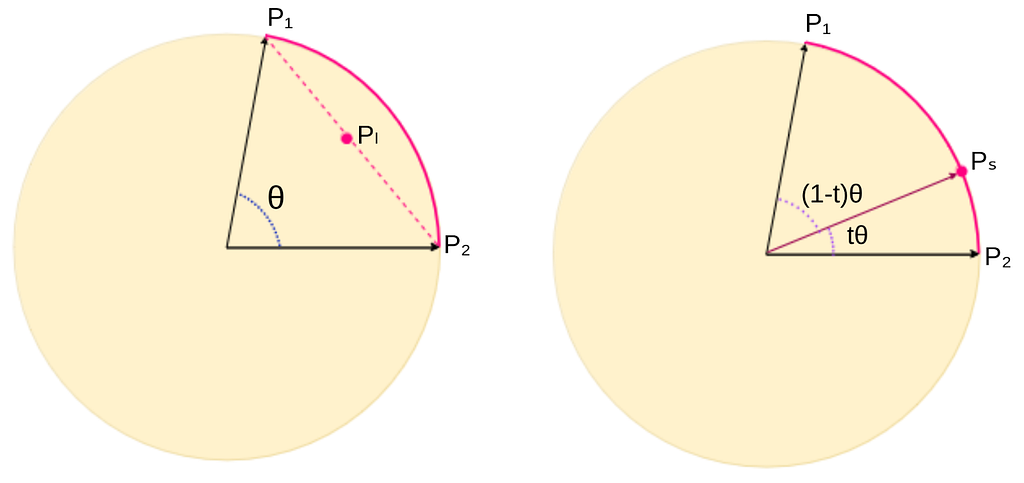
Fig. 2 Pl shows the result of model soup merging while Ps presents the result of SLERP merging (image by authors).
SLERP (Spherical Linear Interpolation, first introduced here) is a technique commonly used in computer graphics and animation for smoothly interpolating between rotations represented by quaternions. SLERP is also applicable in model merging. It merges two sets of model parameters by interpolating along a spherical path instead of a straight line. Fig. 2 shows that for the given two model parameters p1 and p2, SLERP merges these parameters along the globe’s surface, providing a smooth transition. This method is commonly used in merging LLMs.
Assume two MLP models are given, each fine-tuned on a different downstream task. SLERP can merge these two models using the following steps:
Step 1: For each model parameters, flatten and concatenate them into vectors v1, v2
Step 2: Normalize the vectors v1 and v2 to be on the unit hypersphere surface (resulting in v1′ and v2′).
Step 3: Calculate the angle θ (in radians) between these two vectors.
Step 4: Calculate Vslerp using the SLERP formula as:

where t is the interpolation parameter as t=0 means only Model 1 is used, while t=1 means only Model 2 is used.
Linear weight averaging techniques, such as model soup and SLERP, have been common in the field of computer vision from image processing and classification models to image generation models such as latent diffusion models.
Task arithmetic introduces a method based on task vectors. A task vector is calculated by subtracting the weights of a pretrained model (θpre) from the weights of the same model fine-tuned for a specific task (θft), as
τ = θft − θpre. This vector represents a direction in the weight space of the pretrained model where moving in that direction enhances performance on that task. Task vectors can be combined together by arithmetic operations such as negation and addition. Negating a task vector (θpre — τ) reduces the model’s performance on the target task (forgetting) with minimal impact on control tasks. To enhance the performance of the pre-trained model across multiple tasks, we can initially learn a task vector for each task. By then summing these task vectors (θpre+∑τi), we improve the model’s capability to handle multiple tasks simultaneously.
TIES addresses performance drops due to parameter interference when combining task vectors (∑τi). This issue can be solved through three steps (see Fig. 3):
(1) trim each task vector to the top-k% (usually k=20) largest magnitude values,
(2) for each non-zero parameter, select the sign with the highest total magnitude across all task vectors to avoid conflicting changes, and
(3) merging values only from task vectors with the same sign as the elected one.
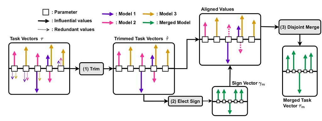
Fig. 3 A depiction of the steps involved in TIES. Each parameter in a model is visualized as a square. The arrows depict the update (task vector, τ ) to a parameter produced by fine-tuning on different tasks (coded by colors), with direction denoting sign and length denoting magnitude. 1- Trim the task vector values based on their magnitude, 2- Elect the sign for each parameter (γm, green vector containing +1 or −1) by resolving sign conflicts, 3- Pick only the values that align with the elected sign and take their mean as the final parameter value. (image from paper)
DARE is mainly focused on LLM’s model merging and identifies the extreme redundancy in the task vector (τ = θft−θpre). It proposes a three step approach:
1- Randomly drop p% (usually p =90) of the task vector values,
2- Rescale the remaining ones by a factor of 1/(1 − p), and
3- Merge (θpre + λi ∑τi)
where λi is the scaling term, representing the importance of each task vector to be merged.
1.b Merging With Data Requirement:
The merging methods that we discussed above require no data. However, there are approaches that do need data to determine the optimal weights for merging the parameters. These methods use data to compute the activations and then adjust the weights accordingly.
One such approach is Fisher Merging. Given K fine-tuned models, each trained on a different downstream task starting from a specific pretrained checkpoint, Fisher Merging performs a weighted summation of each model’s parameters. The weights are calculated using the Fisher information matrix, which requires some data from each task for the matrix construction.
In a related development, RegMean significantly outperforms Fisher-weighted merging by recasting the model merging task as a linear regression problem. This method derives closed-form solutions for the weights of linear layers and interpolates other weights (like layer normalization and bias terms) evenly. Given K fine-tuned models and some data Xi i= 1,..,K, for each task, the linear layers of the merged model can be determined as follows:

Where Wi is the linear layer from the ith fine-tuned model.
2. Merging Models with Identical Architectures but Different Initializations
Given models that have the same architecture and training dataset but different initializations, simple merging methods like linear model combination often fail to perform well. The main reason is that the weights of the models are not aligned. Hence, researchers have developed techniques to leverage the permutation symmetry of neural networks. By reordering the neurons of the models, their weights can align better, which makes the merging process more effective.
Git-Rebasin suggests permuting the weights of one model to match the configuration of another. Assume two models, A and B are given with the same architecture and training dataset, but their initializations and training data orders were different. The weights of each network can be permuted without changing its functionality, which means that swapping neurons in hidden layers can result in functionally equivalent models.
They formulated this as an optimization problem to identify the optimal permutations of units across layers that align the two models’ parameters in the weight space. This alignment ensures that the models are in a similar “basin” of the loss landscape, which leads to a smooth and effective merging. To this goal, Git-Rebasin proposed the following three steps:
1. For each layer, the problem of finding the best permutations is formulated as a Linear Assignment Problem (LAP). This step involves computing a matrix of activations and finding the optimal permutation matrix that aligns the activations.
2. Given the optimal permutations for all layers, the weights of model B will be permuted.
3. Linear model combination between the permuted weights of model B and the weights of model A lies within a low-loss basin in the loss landscape, which ensures that the merged model performs well.
REPAIR addresses a critical issue in the Rebasin merging method known as variance collapse, in which the hidden units have significantly smaller activation variance compared to the corresponding units of the original networks before they were interpolated. Therefore, the activations of neurons become nearly constant in deeper layers, hence the network will no longer even be able to differentiate between inputs. REPAIR resolves this issue by rescaling the activations of the interpolated networks to match the statistical properties of the original networks. By adjusting the means and variances of the activations, the interpolated network maintains functional variability throughout its layers. Applying the REPAIR method significantly reduces the interpolation barrier, improving the performance of interpolated models.
3. Merging Models with Different Architectures
In contrast to the methods discussed so far, Frankenmerging does not fuse models into a single one, and instead stacks different layers of different models sequentially. Therefore, it is able to merge models with different architectures.
For example, to construct an LLM with 40 layers, one might stack the first 24 layers from one LLM onto layers 25–40 from another LLM. This method has gained significant attention in style transfer in computer vision. Despite requiring a lot of trial and error and experimentation, it has led to impressive LLM models such as Goliath and Solar-10.7B [see here].
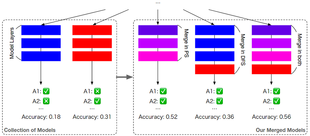
Fig.4 Overview of EvolutionaryOptimization approach (image from paper).
EvolutionaryOptimization proposes a framework to automatically merge a given set of foundation models, such that the merged model outperforms any individual model in the given set. This approach involves two main phases (see Fig. 4):
In the first phase, this method uses TIES-Merging with DARE for layer-wise merging of N foundational models. The process is optimized by using an evolutionary algorithm guided by task-specific metrics (e.g., accuracy for MGSM, ROUGE score for VQA). To find unknown variables such as dropout percentages in DARE and weights of each model’s parameters in merging, the evolutionary optimization begins with a group of possible solutions that evolve over time. Through mutation (small random changes) and crossover (combining parts of two solutions), the best solutions are selected to create a new group of candidates. This iterative process leads to progressively better solutions.
In the second phase, where a set of N models is given, the goal is to find an optimal model with T layers using Frankenmerging. To reduce the search space and make the optimization tractable, all layers are laid out in sequential order (i.e., all layers in the i-th model followed by those in the i + 1-th model) and repeated r times. In this phase, the goal is to find an optimal indicator which determines the inclusion/exclusion of layers: if Indicator(i)>0, the ith layer is included in the merged model; otherwise, it is excluded.
The EvolutionaryOptimization process begins with applying the first phase to a collection of models. Then, the merged model from the first step is added to the given collection and the second phase is applied on this enlarged collection to find an optimal indicator which selects T layers for the final merged model. This approach applied to merge a Japanese LLM with an English Math LLM to build a Japanese Math LLM. The merged model achieved state-of-the-art performance on a variety of established Japanese LLM benchmarks, even outperforming models with significantly more parameters, despite not being trained for such tasks.
References:
[1] Model soup: Wortsman, Mitchell, et al. “Model soups: averaging weights of multiple fine-tuned models improves accuracy without increasing inference time.” (2022).
[2] Task arithmetic: Ilharco, Gabriel, et al. “Editing models with task arithmetic.” (2022).
[3] TIES: Yadav, Prateek, et al. “Ties-merging: Resolving interference when merging models.” (2024).
[4] DARE: Yu, Le, et al. “Language models are super mario: Absorbing abilities from homologous models as a free lunch.” (2024).
[5] Fisher Merging Matena, Michael S., et al. “Merging models with fisher-weighted averaging.” (2022).
[6] RegMean: Jin, Xisen, et al. “Dataless knowledge fusion by merging weights of language models.” (2022).
[7] Git-Rebasin: Ainsworth, Samuel K., et al. “Git re-basin: Merging models modulo permutation symmetries.” (2022).
[8] REPAIR: Jordan, Keller, et al. “Repair: Renormalizing permuted activations for interpolation repair.” (2022).
[9] Frankenmerging: Charles O. Goddard. 2024. mergekit.
[10] EvolutionaryOptimization: Akiba, Takuya, et al. “Evolutionary optimization of model merging recipes.” (2024).
[11] Shoemake, Ken. “Animating rotation with quaternion curves.” (1985).
[12] LMC: Nagarajan, Vaishnavh, et al. “Uniform convergence may be unable to explain generalization in deep learning.” (2019).
[13] Kaddour, Jean, et al. “When do flat minima optimizers work?.” (2022)
[14] Petzka, Henning, et al. “Relative flatness and generalization.” (2021)

Beyond Fine-Tuning: Merging Specialized LLMs Without the Data Burden was originally published in Towards Data Science on Medium, where people are continuing the conversation by highlighting and responding to this story.
Authors: Elahe Aghapour, Salar Rahili
Introduction:
The field of computer vision and natural language processing is evolving rapidly, leading to a growing demand for specialized models fine-tuned for specific downstream tasks. However, having different fine-tuned models has multiple drawbacks:
1. For each task, a separate model must be stored and deployed (this issue can be resolved by applying methods like LoRA for fine-tuning).
2. Independently fine-tuned models cannot benefit from leveraging information from related tasks, which limits their generalization across both in-domain and out-of-domain tasks. However, multi-task learning requires access to datasets for each specific task, and integrating these datasets can be complicated. What if we do not have access to datasets for all downstream tasks, but the fine-tuned models are available? Imagine you need a large language model (LLM) fine-tuned on a set of specific tasks. Instead of collecting extensive datasets for downstream tasks and undergoing the resource-heavy process of fine-tuning, you can find LLMs fine-tuned on each task and merge these models to create the desired one. Note that finding such models is not a difficult task within the large Hugging Face repository, which hosts approximately 0.5 million fine-tuned models. Merging multiple models has recently gained significant attention, primarily because it requires lightweight computation and no training data.

Fig.1 Model ensemble combines outputs from multiple models to boost accuracy but requires more computational resources. Multi-task learning trains one model on several tasks simultaneously, needing access to all datasets and high computational power. Model merging, however, fuses pre-trained models into one, leveraging their strengths with minimal computation and no extra training costs, offering a highly efficient solution (image from paper).
With the growing attention to merging, public libraries such as WEBUI and MergeKit have been developed to facilitate this process. WebUIs enables merging fine-tuned models such as Stable Diffusion using different merging techniques. MergeKit is an open-source, centralized library that offers different merging methods. It facilitates model merging by its efficient implementation of merging techniques, applicable on any hardware.
Here, we categorized merging methods into three main categories:
1. merging models with identical architectures and initializations,
2. merging models with identical architectures but different initializations,
3. merging models with different architectures.
Each category involves different techniques to effectively combine models, which will be explained below.
1. Merging Models with Both Identical Architectures and Initializations:1. merging models with identical architectures and initializations,
2. merging models with identical architectures but different initializations,
3. merging models with different architectures.
Each category involves different techniques to effectively combine models, which will be explained below.
1.a Merging With No Data Requirement:
The model merging methods in this section are all based on Linear Mode Connectivity (LMC). LMC suggests that for models with identical architecture and initialization, the loss between their checkpoints can be connected by a low-loss linear path. This means that these models can be combined using linear interpolation.
To fine-tune a model, various configurations, like different learning rates, random seeds, and data augmentation techniques can be applied which result in different model parameters. Model soup proposes averaging these parameters since these models have learned similar representations and are close in parameter space. Weighted model averaging leads to a flat local optimum with better generalization to out-of-distribution tasks [see 13, 14]

Fig. 2 Pl shows the result of model soup merging while Ps presents the result of SLERP merging (image by authors).
SLERP (Spherical Linear Interpolation, first introduced here) is a technique commonly used in computer graphics and animation for smoothly interpolating between rotations represented by quaternions. SLERP is also applicable in model merging. It merges two sets of model parameters by interpolating along a spherical path instead of a straight line. Fig. 2 shows that for the given two model parameters p1 and p2, SLERP merges these parameters along the globe’s surface, providing a smooth transition. This method is commonly used in merging LLMs.
Assume two MLP models are given, each fine-tuned on a different downstream task. SLERP can merge these two models using the following steps:
Step 1: For each model parameters, flatten and concatenate them into vectors v1, v2
Step 2: Normalize the vectors v1 and v2 to be on the unit hypersphere surface (resulting in v1′ and v2′).
Step 3: Calculate the angle θ (in radians) between these two vectors.
Step 4: Calculate Vslerp using the SLERP formula as:

where t is the interpolation parameter as t=0 means only Model 1 is used, while t=1 means only Model 2 is used.
Linear weight averaging techniques, such as model soup and SLERP, have been common in the field of computer vision from image processing and classification models to image generation models such as latent diffusion models.
Task arithmetic introduces a method based on task vectors. A task vector is calculated by subtracting the weights of a pretrained model (θpre) from the weights of the same model fine-tuned for a specific task (θft), as
τ = θft − θpre. This vector represents a direction in the weight space of the pretrained model where moving in that direction enhances performance on that task. Task vectors can be combined together by arithmetic operations such as negation and addition. Negating a task vector (θpre — τ) reduces the model’s performance on the target task (forgetting) with minimal impact on control tasks. To enhance the performance of the pre-trained model across multiple tasks, we can initially learn a task vector for each task. By then summing these task vectors (θpre+∑τi), we improve the model’s capability to handle multiple tasks simultaneously.
TIES addresses performance drops due to parameter interference when combining task vectors (∑τi). This issue can be solved through three steps (see Fig. 3):
(1) trim each task vector to the top-k% (usually k=20) largest magnitude values,
(2) for each non-zero parameter, select the sign with the highest total magnitude across all task vectors to avoid conflicting changes, and
(3) merging values only from task vectors with the same sign as the elected one.

Fig. 3 A depiction of the steps involved in TIES. Each parameter in a model is visualized as a square. The arrows depict the update (task vector, τ ) to a parameter produced by fine-tuning on different tasks (coded by colors), with direction denoting sign and length denoting magnitude. 1- Trim the task vector values based on their magnitude, 2- Elect the sign for each parameter (γm, green vector containing +1 or −1) by resolving sign conflicts, 3- Pick only the values that align with the elected sign and take their mean as the final parameter value. (image from paper)
DARE is mainly focused on LLM’s model merging and identifies the extreme redundancy in the task vector (τ = θft−θpre). It proposes a three step approach:
1- Randomly drop p% (usually p =90) of the task vector values,
2- Rescale the remaining ones by a factor of 1/(1 − p), and
3- Merge (θpre + λi ∑τi)
where λi is the scaling term, representing the importance of each task vector to be merged.
1.b Merging With Data Requirement:
The merging methods that we discussed above require no data. However, there are approaches that do need data to determine the optimal weights for merging the parameters. These methods use data to compute the activations and then adjust the weights accordingly.
One such approach is Fisher Merging. Given K fine-tuned models, each trained on a different downstream task starting from a specific pretrained checkpoint, Fisher Merging performs a weighted summation of each model’s parameters. The weights are calculated using the Fisher information matrix, which requires some data from each task for the matrix construction.
In a related development, RegMean significantly outperforms Fisher-weighted merging by recasting the model merging task as a linear regression problem. This method derives closed-form solutions for the weights of linear layers and interpolates other weights (like layer normalization and bias terms) evenly. Given K fine-tuned models and some data Xi i= 1,..,K, for each task, the linear layers of the merged model can be determined as follows:

Where Wi is the linear layer from the ith fine-tuned model.
2. Merging Models with Identical Architectures but Different Initializations
Given models that have the same architecture and training dataset but different initializations, simple merging methods like linear model combination often fail to perform well. The main reason is that the weights of the models are not aligned. Hence, researchers have developed techniques to leverage the permutation symmetry of neural networks. By reordering the neurons of the models, their weights can align better, which makes the merging process more effective.
Git-Rebasin suggests permuting the weights of one model to match the configuration of another. Assume two models, A and B are given with the same architecture and training dataset, but their initializations and training data orders were different. The weights of each network can be permuted without changing its functionality, which means that swapping neurons in hidden layers can result in functionally equivalent models.
They formulated this as an optimization problem to identify the optimal permutations of units across layers that align the two models’ parameters in the weight space. This alignment ensures that the models are in a similar “basin” of the loss landscape, which leads to a smooth and effective merging. To this goal, Git-Rebasin proposed the following three steps:
1. For each layer, the problem of finding the best permutations is formulated as a Linear Assignment Problem (LAP). This step involves computing a matrix of activations and finding the optimal permutation matrix that aligns the activations.
2. Given the optimal permutations for all layers, the weights of model B will be permuted.
3. Linear model combination between the permuted weights of model B and the weights of model A lies within a low-loss basin in the loss landscape, which ensures that the merged model performs well.
REPAIR addresses a critical issue in the Rebasin merging method known as variance collapse, in which the hidden units have significantly smaller activation variance compared to the corresponding units of the original networks before they were interpolated. Therefore, the activations of neurons become nearly constant in deeper layers, hence the network will no longer even be able to differentiate between inputs. REPAIR resolves this issue by rescaling the activations of the interpolated networks to match the statistical properties of the original networks. By adjusting the means and variances of the activations, the interpolated network maintains functional variability throughout its layers. Applying the REPAIR method significantly reduces the interpolation barrier, improving the performance of interpolated models.
3. Merging Models with Different Architectures
In contrast to the methods discussed so far, Frankenmerging does not fuse models into a single one, and instead stacks different layers of different models sequentially. Therefore, it is able to merge models with different architectures.
For example, to construct an LLM with 40 layers, one might stack the first 24 layers from one LLM onto layers 25–40 from another LLM. This method has gained significant attention in style transfer in computer vision. Despite requiring a lot of trial and error and experimentation, it has led to impressive LLM models such as Goliath and Solar-10.7B [see here].

Fig.4 Overview of EvolutionaryOptimization approach (image from paper).
EvolutionaryOptimization proposes a framework to automatically merge a given set of foundation models, such that the merged model outperforms any individual model in the given set. This approach involves two main phases (see Fig. 4):
In the first phase, this method uses TIES-Merging with DARE for layer-wise merging of N foundational models. The process is optimized by using an evolutionary algorithm guided by task-specific metrics (e.g., accuracy for MGSM, ROUGE score for VQA). To find unknown variables such as dropout percentages in DARE and weights of each model’s parameters in merging, the evolutionary optimization begins with a group of possible solutions that evolve over time. Through mutation (small random changes) and crossover (combining parts of two solutions), the best solutions are selected to create a new group of candidates. This iterative process leads to progressively better solutions.
In the second phase, where a set of N models is given, the goal is to find an optimal model with T layers using Frankenmerging. To reduce the search space and make the optimization tractable, all layers are laid out in sequential order (i.e., all layers in the i-th model followed by those in the i + 1-th model) and repeated r times. In this phase, the goal is to find an optimal indicator which determines the inclusion/exclusion of layers: if Indicator(i)>0, the ith layer is included in the merged model; otherwise, it is excluded.
The EvolutionaryOptimization process begins with applying the first phase to a collection of models. Then, the merged model from the first step is added to the given collection and the second phase is applied on this enlarged collection to find an optimal indicator which selects T layers for the final merged model. This approach applied to merge a Japanese LLM with an English Math LLM to build a Japanese Math LLM. The merged model achieved state-of-the-art performance on a variety of established Japanese LLM benchmarks, even outperforming models with significantly more parameters, despite not being trained for such tasks.
The opinions expressed in this blog post are solely our own and do not reflect those of our employer.
Also Read Our Previous Post: From Unimodals to Multimodality: DIY Techniques for Building Foundational Models
References:
[1] Model soup: Wortsman, Mitchell, et al. “Model soups: averaging weights of multiple fine-tuned models improves accuracy without increasing inference time.” (2022).
[2] Task arithmetic: Ilharco, Gabriel, et al. “Editing models with task arithmetic.” (2022).
[3] TIES: Yadav, Prateek, et al. “Ties-merging: Resolving interference when merging models.” (2024).
[4] DARE: Yu, Le, et al. “Language models are super mario: Absorbing abilities from homologous models as a free lunch.” (2024).
[5] Fisher Merging Matena, Michael S., et al. “Merging models with fisher-weighted averaging.” (2022).
[6] RegMean: Jin, Xisen, et al. “Dataless knowledge fusion by merging weights of language models.” (2022).
[7] Git-Rebasin: Ainsworth, Samuel K., et al. “Git re-basin: Merging models modulo permutation symmetries.” (2022).
[8] REPAIR: Jordan, Keller, et al. “Repair: Renormalizing permuted activations for interpolation repair.” (2022).
[9] Frankenmerging: Charles O. Goddard. 2024. mergekit.
[10] EvolutionaryOptimization: Akiba, Takuya, et al. “Evolutionary optimization of model merging recipes.” (2024).
[11] Shoemake, Ken. “Animating rotation with quaternion curves.” (1985).
[12] LMC: Nagarajan, Vaishnavh, et al. “Uniform convergence may be unable to explain generalization in deep learning.” (2019).
[13] Kaddour, Jean, et al. “When do flat minima optimizers work?.” (2022)
[14] Petzka, Henning, et al. “Relative flatness and generalization.” (2021)
Beyond Fine-Tuning: Merging Specialized LLMs Without the Data Burden was originally published in Towards Data Science on Medium, where people are continuing the conversation by highlighting and responding to this story.
