10 Applications of vector search to deeply understand your data and models

Artistic rendering of vector search for data exploration. Image generated by DALLE-3.
As large language models (LLMs) have eaten the world, vector search engines have tagged along for the ride. Vector databases form the foundation of the long-term memory systems for LLMs.
By efficiently finding relevant information to pass in as context to the language model, vector search engines can provide up-to-date information beyond the training cutoff and enhance the quality of the model’s output without fine-tuning. This process, commonly referred to as retrieval augmented generation (RAG), has thrust the once-esoteric algorithmic challenge of approximate nearest neighbor (ANN) search into the spotlight!
Amidst all of the commotion, one could be forgiven for thinking that vector search engines are inextricably linked to large language models. But there’s so much more to the story. Vector search has a plethora of powerful applications that go well beyond improving RAG for LLMs!
In this article, I will show you ten of my favorite uses of vector search for data understanding, data exploration, model interpretability and more.
Here are the applications we will cover, in roughly increasing order of complexity:
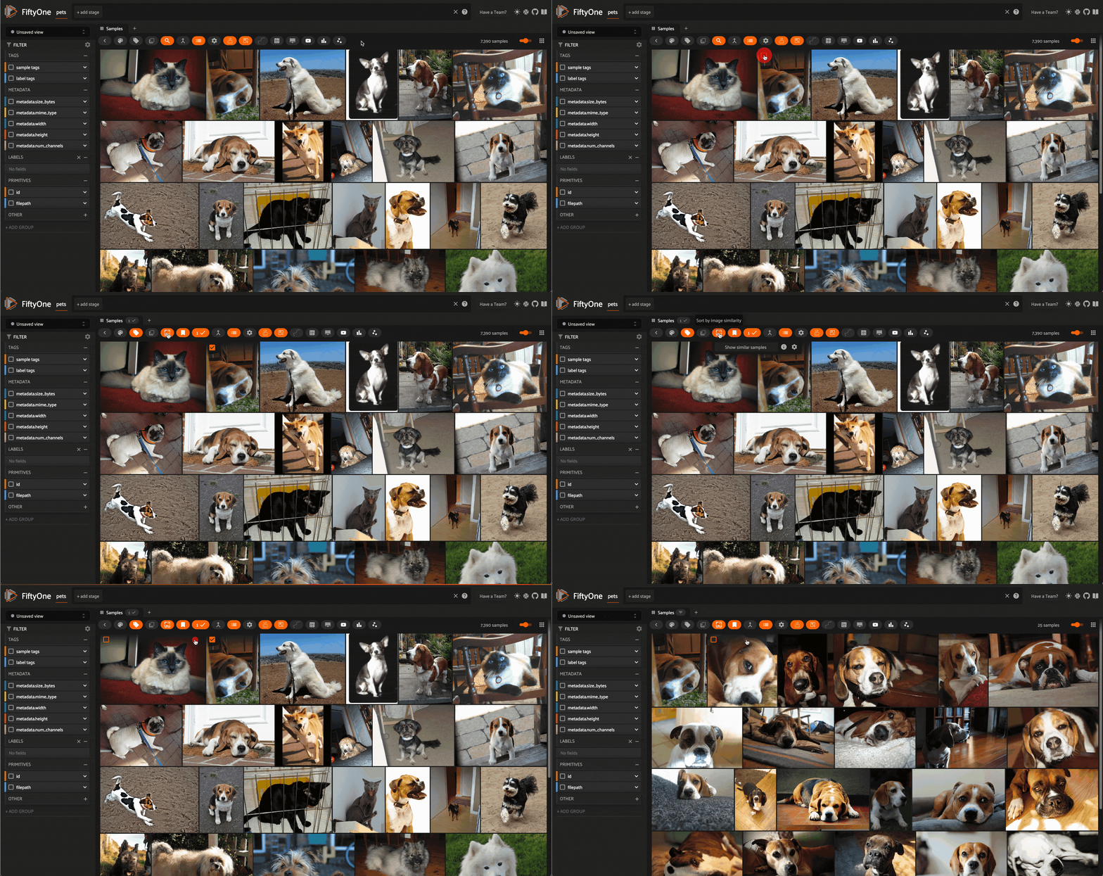
Image similarity search on images from the Oxford-IIIT Pet Dataset (LICENSE). Image courtesy of the author.
Perhaps the simplest place to start is image similarity search. In this task, you have a dataset consisting of images — this can be anything from a personal photo album to a massive repository of billions of images captured by thousands of distributed cameras over the course of years.
The setup is simple: compute embeddings for every image in this dataset, and generate a vector index out of these embedding vectors. After this initial batch of computation, no further inference is required. A great way to explore the structure of your dataset is to select an image from the dataset and query the vector index for the k nearest neighbors — the most similar images. This can provide an intuitive sense for how densely the space of images is populated around query images.
For more information and working code, see here.
Reverse Image Search
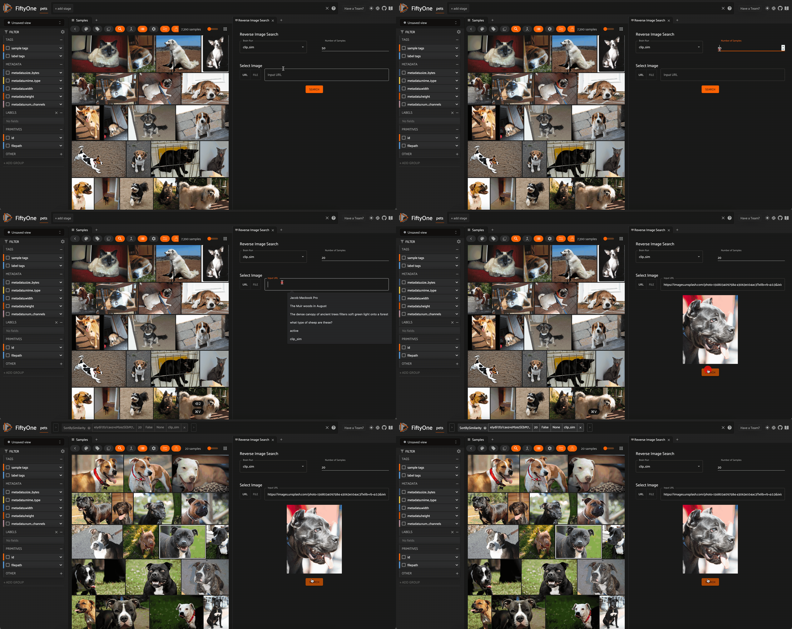
Reverse image search on an image from Unsplash (courtesy Mladen Šćekić) against the Oxford-IIIT Pet Dataset. Image courtesy of the author.
In a similar vein, a natural extension of image similarity search is to find the most similar images within the dataset to an external image. This can be an image from your local filesystem, or an image from the internet!
To perform a reverse image search, you create the vector index for the dataset as in the image similarity search example. The difference comes at run-time, when you compute the embedding for the query image, and then query the vector database with this vector.
For more information and working code, see here.
Object Similarity Search
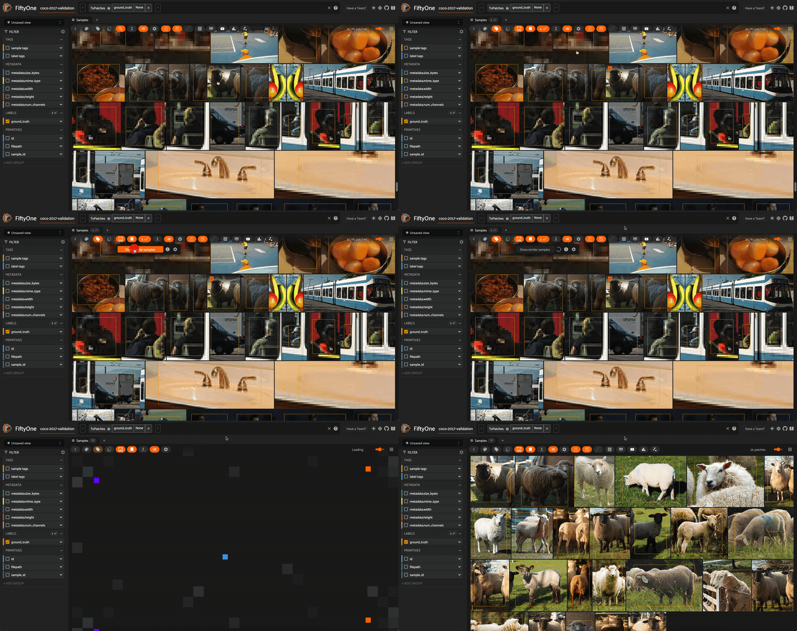
Object similarity search for sheep in the COCO-2017 dataset’s validation split (LICENSE). Image courtesy of the author.
If you want to delve deeper into the content within the images, then object, or “patch” similarity search may be what you’re after. One example of this is person re-identification, where you have a single image with a person of interest in it, and you want to find all instances of that person across your dataset.
The person may only take up small portions of each image, so the embeddings for the entire images they are in might depend strongly on the other content in these images. For instance, there might be multiple people in an image.
A better solution is to treat each object detection patch as if it were a separate entity and compute an embedding for each. Then, create a vector index with these patch embeddings, and run a similarity search against a patch of the person you want to re-identify. As a starting point you may want to try using a ResNet model.
Two subtleties here:
For more information and working code, see here.
Robust OCR Document Search

Fuzzy/semantic search through blocks of text generated by the Tesseract OCR engine on the pages of my Ph.D. thesis. Embeddings computed using GTE-base model. Image courtesy of the author.
Optical Character Recognition (OCR) is a technique that allows you to digitize documents like handwritten notes, old journal articles, medical records, and those love letters squirreled away in your closet. OCR engines like Tesseract and PaddleOCR work by identifying individual characters and symbols in images and creating contiguous “blocks” of text — think paragraphs.
Once you have this text, you can then perform traditional natural language keyword searches over the predicted blocks of text, as illustrated here. However, this method of search is susceptible to single-character errors. If the OCR engine accidentally recognizes an “l” as a “1”, a keyword search for “control” would fail (how about that irony!).
We can overcome this challenge using vector search! Embed the blocks of text using a text embedding model like GTE-base from Hugging Face’s Sentence Transformers library, and create a vector index. We can then perform fuzzy and/or semantic search across our digitized documents by embedding the search text and querying the index. At a high level, the blocks of text within these documents are analogous to the object detection patches in object similarity searches!
For more information and working code, see here.
Semantic Search

Semantic image search using natural language on the COCO 2017 validation split. Image courtesy of the author.
With multimodal models, we can extend the notion of semantic search from text to images. Models like CLIP, OpenCLIP, and MetaCLIP were trained to find common representations of images and their captions, so that the embedding vector for an image of a dog would be very similar to the embedding vector for the text prompt “a photo of a dog”.
This means that it is sensible (i.e. we are “allowed”) to create a vector index out of the CLIP embeddings for the images in our dataset and then run a vector search query against this vector database where the query vector is the CLIP embedding of a text prompt.
?By treating the individual frames in a video as images and adding each frame’s embedding to a vector index, you can also semantically search through videos!
For more information and working code, see here.
Cross-modal Retrieval
In a sense, semantically searching through a dataset of images is a form of cross-modal retrieval. One way of conceptualizing it is that we are retrieving images corresponding to a text query. With models like ImageBind, we can take this a step further!
ImageBind embeds data from six different modalities in the same embedding space: images, text, audio, depth, thermal, and inertial measurement unit (IMU). That means that we can generate a vector index for data in any of these modalities and query this index with a sample of any other of these modalities. For instance, we can take an audio clip of a car honking and retrieve all images of cars!
For more information and working code, see here.
Probing Perceptual Similarity
One very important part of the vector search story which we have only glossed over thus far is the model. The elements in our vector index are embeddings from a model. These embeddings can be the final output of a tailored embedding model, or they can be hidden or latent representations from a model trained on another task like classification.
Regardless, the model we use to embed our samples can have a substantial impact on which samples are deemed most similar to which other samples. A CLIP model captures semantic concepts, but struggles to represent structural information within images. A ResNet model on the other hand is very good at representing similarity in structure and layout, operating on the level of pixels and patches. Then there are embedding models like DreamSim, which aim to bridge the gap and capture mid-level similarity — aligning the model’s notion of similarity with what is perceived by humans.
Vector search provides a way for us to probe how a model is “seeing” the world. By creating a separate vector index for each model we are interested in (on the same data), we can rapidly develop an intuition for how different models are representing data under the hood, so to speak.
Here is an example showcasing similarity searches with CLIP, ResNet, and DreamSim model embeddings for the same query image on the NIGHTS dataset:

Similarity search with ResNet50 embeddings on an image in the NIGHTS dataset (Images generated by Stable Diffusion — MIT RAIL LICENSE). ResNet models operate on the level of pixels and patches. Hence the retrieved images are structurally similar to the query but not always semantically similar.

Similarity search with CLIP embeddings on the same query image. CLIP models respect the underlying semantics of the images but not their layout.

Similarity search with DreamSim embeddings on the same query image. DreamSim bridges the gap, seeking the best mid-level similarity compromise between semantic and structural features.
For more information and working code, see here.
Comparing Model Representations
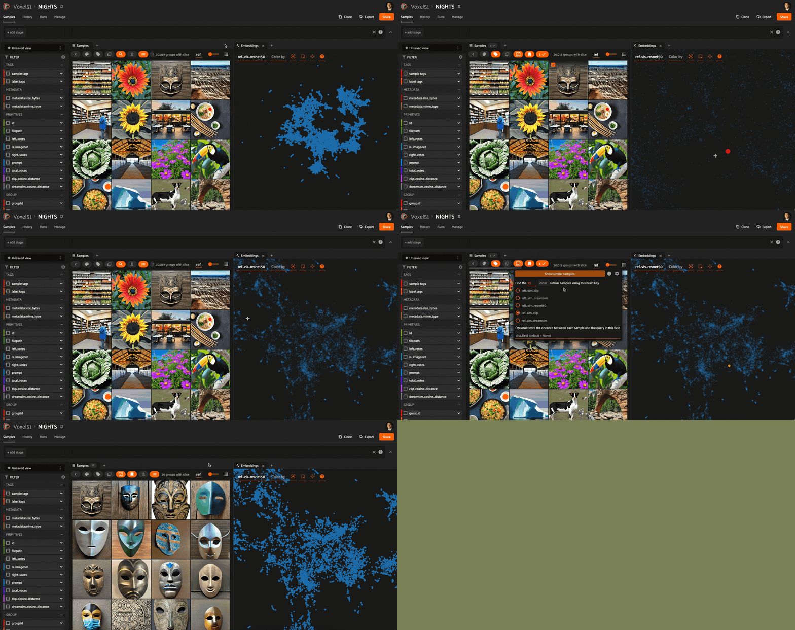
Heuristic comparison of ResNet50 and CLIP model representations of the NIGHTS dataset. ResNet embeddings have been reduced to 2D using UMAP. Selecting a point in the embeddings plot and highlighting nearby samples, we can see how ResNet captures compositional and palette similarity, not semantic similarity. Running a vector search on the selected sample with CLIP embeddings, we can see that the most samples according to CLIP are not localized according to ResNet.
We can gain new insight into the differences between two models by combining vector search and dimensionality reduction techniques like uniform manifold approximation (UMAP). Here’s how:
Each model’s embeddings contain information about how the model is representing the data. Using UMAP (or t-SNE or PCA), we can generate lower dimensional (either 2D or 3D) representations of the embeddings from model1. By doing so, we sacrifice some detail, but hopefully preserve some information about which samples are perceived as similar to other samples. What we gain is the ability to visualize this data.
With model1’s embedding visualization as a backdrop, we can choose a point in this plot and perform a vector search query on that sample with respect to model2’s embeddings. You can then see where within the 2D visualization the retrieved points lie!
The example above uses the same NIGHTS dataset as in the last section, visualizing ResNet embeddings, which capture more compositional and structural similarity, and performing a similarity search with CLIP (semantic) embeddings.
Concept Interpolation
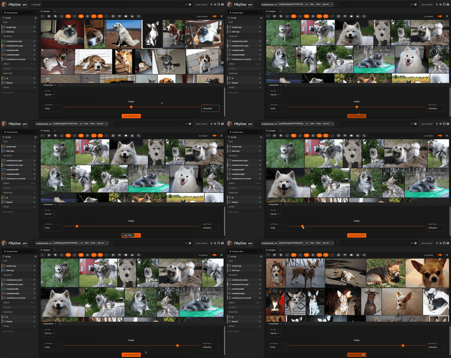
Interpolation between the concepts “husky” and “chihuahua” with CLIP embeddings on the Oxford-IIIT Pet Dataset
We’re reaching the end of the ten applications, but lucky for you I saved a few of the best for last. So far, the only vectors we’ve worked with are embeddings — the vector index is populated with embeddings, and the query vectors are also embeddings. But sometimes there is additional structure in the space of embeddings that we can leverage to interact with our data more dynamically.
One example of such a dynamic interaction is something I like to call “concept interpolation”. Here’s how it works: take a dataset of images and generate a vector index using a multimodal model (text and image). Pick two text prompts like “sunny” and “rainy”, which stand in for concepts, and set a value alpha in the range [0,1]. We can generate the embedding vectors for each text concept, and add these vectors in a linear combination specified by alpha. We then normalize the vector and use it as the query to our vector index of image embeddings.
Because we are linearly interpolating between the embedding vectors for the two text prompts (concepts), we are in a very loose sense interpolating between the concepts themselves! We can dynamically change alpha and query our vector database each time there is an interaction.
?This notion of concept interpolation is experimental (read: not always a well defined operation). I find it works best when the text prompts are conceptually related and the dataset is diverse enough to have different results for different places along the interpolation spectrum.
For more information and working code, see here.
Concept Space Traversal

Traversing the space of “concepts” by moving in the direction of various text prompts via their embeddings, illustrated for the test split of the COCO 2017 dataset. Images and text embedded with a CLIP model. Image courtesy of the author.
Last, but certainly not least, we have what I like to call “concept space traversal”. As with concept interpolation, start with a dataset of images and generate embeddings with a multimodal model like CLIP. Next, select an image from the dataset. This image will serve as your starting point, from which you will be “traversing” the space of concepts.
From there, you can define a direction you want to move in by providing a text string as a stand-in for a concept. Set the magnitude of the “step” you want to take in that direction, and that text string’s embedding vector (with a multiplicative coefficient) will be added to the embedding vector of the initial image. The “destination” vector will be used to query the vector database. You can add arbitrarily many concepts in arbitrary quantities, and watch as the set of retrieved images updates in real time.
As with “concept interpolation”, this is not always a strictly well-defined process. However, I find it to be captivating, and to perform reasonably well when the coefficient applied to the text embeddings is high enough that they are sufficiently taken into account.
For more information and working code, see here.
Conclusion
Vector search engines are incredibly powerful tools. Sure, they are the stars of the best show in town, RAG-time. But vector databases are far more versatile than that. They enable deeper understanding of data, give insights into how models represent that data, and offer new avenues for us to interact with our data.
Vector databases are not bound to LLMs. They prove useful whenever embeddings are involved, and embeddings lie right at the intersection of model and data. The more rigorously we understand the structure of embedding spaces, the more dynamic and pervasive our vector search-enabled data and model interactions will become.
If you found this post interesting, you may also want to check out these vector search powered posts:

From RAGs to Riches was originally published in Towards Data Science on Medium, where people are continuing the conversation by highlighting and responding to this story.

Artistic rendering of vector search for data exploration. Image generated by DALLE-3.
As large language models (LLMs) have eaten the world, vector search engines have tagged along for the ride. Vector databases form the foundation of the long-term memory systems for LLMs.
By efficiently finding relevant information to pass in as context to the language model, vector search engines can provide up-to-date information beyond the training cutoff and enhance the quality of the model’s output without fine-tuning. This process, commonly referred to as retrieval augmented generation (RAG), has thrust the once-esoteric algorithmic challenge of approximate nearest neighbor (ANN) search into the spotlight!
Amidst all of the commotion, one could be forgiven for thinking that vector search engines are inextricably linked to large language models. But there’s so much more to the story. Vector search has a plethora of powerful applications that go well beyond improving RAG for LLMs!
In this article, I will show you ten of my favorite uses of vector search for data understanding, data exploration, model interpretability and more.
Here are the applications we will cover, in roughly increasing order of complexity:
- Image Similarity Search
- Reverse Image Search
- Object Similarity Search
- Robust OCR Document Search
- Semantic Search
- Cross-modal Retrieval
- Probing Perceptual Similarity
- Comparing Model Representations
- Concept Interpolation
- Concept Space Traversal

Image similarity search on images from the Oxford-IIIT Pet Dataset (LICENSE). Image courtesy of the author.
Perhaps the simplest place to start is image similarity search. In this task, you have a dataset consisting of images — this can be anything from a personal photo album to a massive repository of billions of images captured by thousands of distributed cameras over the course of years.
The setup is simple: compute embeddings for every image in this dataset, and generate a vector index out of these embedding vectors. After this initial batch of computation, no further inference is required. A great way to explore the structure of your dataset is to select an image from the dataset and query the vector index for the k nearest neighbors — the most similar images. This can provide an intuitive sense for how densely the space of images is populated around query images.
For more information and working code, see here.
Reverse Image Search

Reverse image search on an image from Unsplash (courtesy Mladen Šćekić) against the Oxford-IIIT Pet Dataset. Image courtesy of the author.
In a similar vein, a natural extension of image similarity search is to find the most similar images within the dataset to an external image. This can be an image from your local filesystem, or an image from the internet!
To perform a reverse image search, you create the vector index for the dataset as in the image similarity search example. The difference comes at run-time, when you compute the embedding for the query image, and then query the vector database with this vector.
For more information and working code, see here.
Object Similarity Search

Object similarity search for sheep in the COCO-2017 dataset’s validation split (LICENSE). Image courtesy of the author.
If you want to delve deeper into the content within the images, then object, or “patch” similarity search may be what you’re after. One example of this is person re-identification, where you have a single image with a person of interest in it, and you want to find all instances of that person across your dataset.
The person may only take up small portions of each image, so the embeddings for the entire images they are in might depend strongly on the other content in these images. For instance, there might be multiple people in an image.
A better solution is to treat each object detection patch as if it were a separate entity and compute an embedding for each. Then, create a vector index with these patch embeddings, and run a similarity search against a patch of the person you want to re-identify. As a starting point you may want to try using a ResNet model.
Two subtleties here:
- In the vector index, you need to store metadata that maps each patch back to its corresponding image in the dataset.
- You will need to run an object detection model to generate these detection patches before instantiating the index. You may also want to only compute patch embeddings for certain classes of objects, like person, and not others — chair, table, etc.
For more information and working code, see here.
Robust OCR Document Search

Fuzzy/semantic search through blocks of text generated by the Tesseract OCR engine on the pages of my Ph.D. thesis. Embeddings computed using GTE-base model. Image courtesy of the author.
Optical Character Recognition (OCR) is a technique that allows you to digitize documents like handwritten notes, old journal articles, medical records, and those love letters squirreled away in your closet. OCR engines like Tesseract and PaddleOCR work by identifying individual characters and symbols in images and creating contiguous “blocks” of text — think paragraphs.
Once you have this text, you can then perform traditional natural language keyword searches over the predicted blocks of text, as illustrated here. However, this method of search is susceptible to single-character errors. If the OCR engine accidentally recognizes an “l” as a “1”, a keyword search for “control” would fail (how about that irony!).
We can overcome this challenge using vector search! Embed the blocks of text using a text embedding model like GTE-base from Hugging Face’s Sentence Transformers library, and create a vector index. We can then perform fuzzy and/or semantic search across our digitized documents by embedding the search text and querying the index. At a high level, the blocks of text within these documents are analogous to the object detection patches in object similarity searches!
For more information and working code, see here.
Semantic Search

Semantic image search using natural language on the COCO 2017 validation split. Image courtesy of the author.
With multimodal models, we can extend the notion of semantic search from text to images. Models like CLIP, OpenCLIP, and MetaCLIP were trained to find common representations of images and their captions, so that the embedding vector for an image of a dog would be very similar to the embedding vector for the text prompt “a photo of a dog”.
This means that it is sensible (i.e. we are “allowed”) to create a vector index out of the CLIP embeddings for the images in our dataset and then run a vector search query against this vector database where the query vector is the CLIP embedding of a text prompt.
?By treating the individual frames in a video as images and adding each frame’s embedding to a vector index, you can also semantically search through videos!
For more information and working code, see here.
Cross-modal Retrieval
In a sense, semantically searching through a dataset of images is a form of cross-modal retrieval. One way of conceptualizing it is that we are retrieving images corresponding to a text query. With models like ImageBind, we can take this a step further!
ImageBind embeds data from six different modalities in the same embedding space: images, text, audio, depth, thermal, and inertial measurement unit (IMU). That means that we can generate a vector index for data in any of these modalities and query this index with a sample of any other of these modalities. For instance, we can take an audio clip of a car honking and retrieve all images of cars!
For more information and working code, see here.
Probing Perceptual Similarity
One very important part of the vector search story which we have only glossed over thus far is the model. The elements in our vector index are embeddings from a model. These embeddings can be the final output of a tailored embedding model, or they can be hidden or latent representations from a model trained on another task like classification.
Regardless, the model we use to embed our samples can have a substantial impact on which samples are deemed most similar to which other samples. A CLIP model captures semantic concepts, but struggles to represent structural information within images. A ResNet model on the other hand is very good at representing similarity in structure and layout, operating on the level of pixels and patches. Then there are embedding models like DreamSim, which aim to bridge the gap and capture mid-level similarity — aligning the model’s notion of similarity with what is perceived by humans.
Vector search provides a way for us to probe how a model is “seeing” the world. By creating a separate vector index for each model we are interested in (on the same data), we can rapidly develop an intuition for how different models are representing data under the hood, so to speak.
Here is an example showcasing similarity searches with CLIP, ResNet, and DreamSim model embeddings for the same query image on the NIGHTS dataset:

Similarity search with ResNet50 embeddings on an image in the NIGHTS dataset (Images generated by Stable Diffusion — MIT RAIL LICENSE). ResNet models operate on the level of pixels and patches. Hence the retrieved images are structurally similar to the query but not always semantically similar.

Similarity search with CLIP embeddings on the same query image. CLIP models respect the underlying semantics of the images but not their layout.

Similarity search with DreamSim embeddings on the same query image. DreamSim bridges the gap, seeking the best mid-level similarity compromise between semantic and structural features.
For more information and working code, see here.
Comparing Model Representations

Heuristic comparison of ResNet50 and CLIP model representations of the NIGHTS dataset. ResNet embeddings have been reduced to 2D using UMAP. Selecting a point in the embeddings plot and highlighting nearby samples, we can see how ResNet captures compositional and palette similarity, not semantic similarity. Running a vector search on the selected sample with CLIP embeddings, we can see that the most samples according to CLIP are not localized according to ResNet.
We can gain new insight into the differences between two models by combining vector search and dimensionality reduction techniques like uniform manifold approximation (UMAP). Here’s how:
Each model’s embeddings contain information about how the model is representing the data. Using UMAP (or t-SNE or PCA), we can generate lower dimensional (either 2D or 3D) representations of the embeddings from model1. By doing so, we sacrifice some detail, but hopefully preserve some information about which samples are perceived as similar to other samples. What we gain is the ability to visualize this data.
With model1’s embedding visualization as a backdrop, we can choose a point in this plot and perform a vector search query on that sample with respect to model2’s embeddings. You can then see where within the 2D visualization the retrieved points lie!
The example above uses the same NIGHTS dataset as in the last section, visualizing ResNet embeddings, which capture more compositional and structural similarity, and performing a similarity search with CLIP (semantic) embeddings.
Concept Interpolation

Interpolation between the concepts “husky” and “chihuahua” with CLIP embeddings on the Oxford-IIIT Pet Dataset
We’re reaching the end of the ten applications, but lucky for you I saved a few of the best for last. So far, the only vectors we’ve worked with are embeddings — the vector index is populated with embeddings, and the query vectors are also embeddings. But sometimes there is additional structure in the space of embeddings that we can leverage to interact with our data more dynamically.
One example of such a dynamic interaction is something I like to call “concept interpolation”. Here’s how it works: take a dataset of images and generate a vector index using a multimodal model (text and image). Pick two text prompts like “sunny” and “rainy”, which stand in for concepts, and set a value alpha in the range [0,1]. We can generate the embedding vectors for each text concept, and add these vectors in a linear combination specified by alpha. We then normalize the vector and use it as the query to our vector index of image embeddings.
Because we are linearly interpolating between the embedding vectors for the two text prompts (concepts), we are in a very loose sense interpolating between the concepts themselves! We can dynamically change alpha and query our vector database each time there is an interaction.
?This notion of concept interpolation is experimental (read: not always a well defined operation). I find it works best when the text prompts are conceptually related and the dataset is diverse enough to have different results for different places along the interpolation spectrum.
For more information and working code, see here.
Concept Space Traversal

Traversing the space of “concepts” by moving in the direction of various text prompts via their embeddings, illustrated for the test split of the COCO 2017 dataset. Images and text embedded with a CLIP model. Image courtesy of the author.
Last, but certainly not least, we have what I like to call “concept space traversal”. As with concept interpolation, start with a dataset of images and generate embeddings with a multimodal model like CLIP. Next, select an image from the dataset. This image will serve as your starting point, from which you will be “traversing” the space of concepts.
From there, you can define a direction you want to move in by providing a text string as a stand-in for a concept. Set the magnitude of the “step” you want to take in that direction, and that text string’s embedding vector (with a multiplicative coefficient) will be added to the embedding vector of the initial image. The “destination” vector will be used to query the vector database. You can add arbitrarily many concepts in arbitrary quantities, and watch as the set of retrieved images updates in real time.
As with “concept interpolation”, this is not always a strictly well-defined process. However, I find it to be captivating, and to perform reasonably well when the coefficient applied to the text embeddings is high enough that they are sufficiently taken into account.
For more information and working code, see here.
Conclusion
Vector search engines are incredibly powerful tools. Sure, they are the stars of the best show in town, RAG-time. But vector databases are far more versatile than that. They enable deeper understanding of data, give insights into how models represent that data, and offer new avenues for us to interact with our data.
Vector databases are not bound to LLMs. They prove useful whenever embeddings are involved, and embeddings lie right at the intersection of model and data. The more rigorously we understand the structure of embedding spaces, the more dynamic and pervasive our vector search-enabled data and model interactions will become.
If you found this post interesting, you may also want to check out these vector search powered posts:
- ? How I Turned My Company’s Docs into a Searchable Database with OpenAI
- ? How I Turned ChatGPT into an SQL-Like Translator for Image and Video Datasets
- ? What I Learned Pushing Prompt Engineering to the Limit
From RAGs to Riches was originally published in Towards Data Science on Medium, where people are continuing the conversation by highlighting and responding to this story.
