How can you get a computer to distinguish between different types of objects in an image? A step-by-step guide.
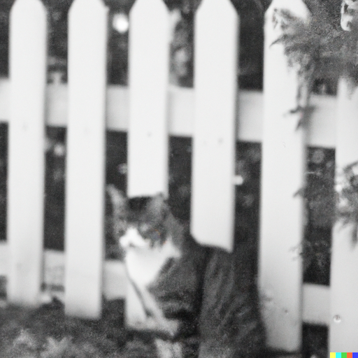
An image of a cat in front of a white picket fence. From DALL·E 3.
Table of Contents
Relevant Links
Image segmentation refers to the ability of computers (or more accurately models stored on computers) to take an image and assign each pixel in the image to a corresponding category. For example, it is possible to run the image of a cat in front of a white fence shown above through an image segmenter and have it spit out the segmented image below:
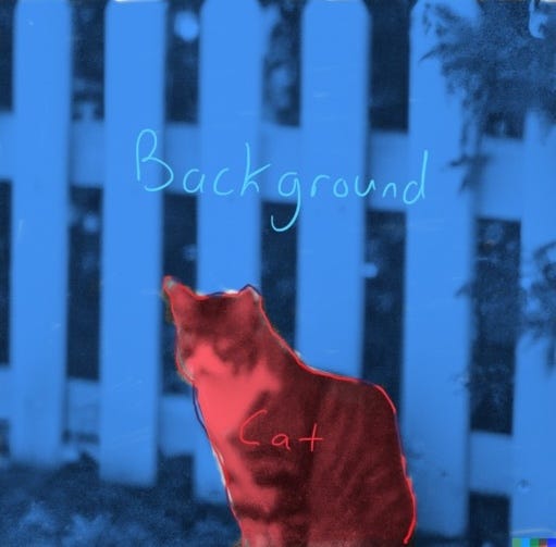
The cat image, segmented into ‘cat’ pixels and ‘background’ pixels. Modified image from DALL·E 3.
In this example, I segmented the image by hand. This is a tedious operation, and one that we would love to automate. In this guide I will walk you through the process of training an algorithm to conduct image segmentation. Many guides on the internet and in textbooks are helpful to a certain extent, but they all fail to go into the nitty gritty details of the implementation. Here I will leave as few stones unturned as possible, to help you save time when implementing image segmentation on your own datasets.
First, let us place our task in the broader context of machine learning. The definition of machine learning is self-evident: we are teaching machines to learn how to solve problems that we would love to automate. There are many problems humans would like to automate; in this article we focus on a subset of problems in computer vision. Computer vision seeks to teach a computer how to see. It is trivial to give a six-year-old child an image of a cat in front of a white picket fence and ask them to segment the image into ‘cat’ pixels and ‘background’ pixels (after you explain what ‘segment’ means to the confused child, of course.) And yet for decades computers have struggled mightily with this problem.
Why do computers struggle to do what a six-year-old can do? We can empathize with the computer by thinking about how one learns to read via braille. Imagine you are handed an essay written in braille, and assume you have no knowledge of how to read it. How would you proceed? What would you need to decipher the braille into English?
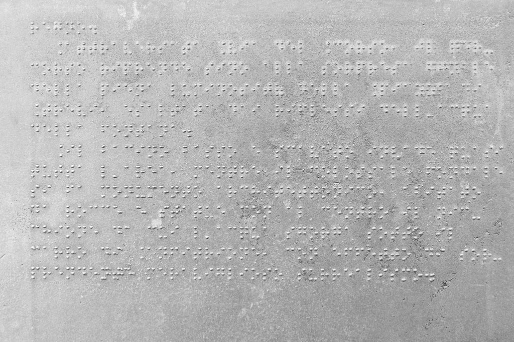
A small passage written in braille. From Unsplash.
What you require is a method of transforming this input into an output that is legible to you. In mathematics we call this a mapping. We say that we would like to learn a function f(x) that maps our input x that is illegible into an output y that is legible.

With many months of practice and a good tutor, anyone can learn the necessary mapping from braille to English. By analogy, a computer processing an image is a bit like someone encountering braille for the first time; it appears like a bunch of nonsense. The computer needs to learn the necessary mapping f(x) to transform a bunch of numbers corresponding to pixels into something that it can use to segment the image. And unfortunately the computer model doesn’t have thousands of years of evolution, biology, and years of experience seeing the world; it is essentially ‘born’ when you start up your program. This is what we hope to teach our model in computer vision.
Why would we want to conduct image segmentation in the first place? One of the more obvious use cases is Zoom. Many people favor using virtual backgrounds when video conferencing to avoid having their co-workers see their dog doing cartwheels in the living room. Image segmentation is crucial to this task. Another powerful use case is medical imaging. When taking CT scans of patient’s organs, it could be helpful to have an algorithm automatically segment the organs in the images so that medical professionals can determine things like injury, the presence of tumors, etc. Here is a great example of a Kaggle competition focused on this task.
There are several flavors of image segmentation, ranging from simple to complex. In this article we will be dealing with the simplest kind of image segmentation: binary segmentation. This means that there will only be two different classes of objects e.g. ‘cat’ and ‘background’. No more, no less.
Note that the code I present here has been slightly rearranged and edited for clarity. To run some working code, please see links to code at the top of the article. We will be using the Carvana Image Masking Challenge dataset from Kaggle. You will need to sign up for this challenge to get access the dataset, and plug in your Kaggle API key into the Colab notebook to get it to work (if you don’t want to use the Kaggle notebook). Please see this discussion post for details on how to do this.
One more thing; as much as I would like to dive into detail on every idea in this code, I will presume you have some working knowledge of convolutional neural networks, max pooling layers, densely connected layers, dropout layers, and residual connectors. Unfortunately discussing these concepts at length would require a new article, and is outside the scope of this one, where we focus on the nuts and bolts of implementation.
Extracting Data
The relevant data for this article will be housed in the following folders:
In the context of image segmentation, a mask is the segmented image. We are trying to get our model to learn how to map an input image to an output segmentation mask. It is usually assumed that the true mask (a.k.a. ground truth) is hand-drawn by a human expert.
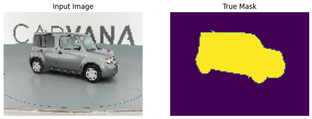
An example of an image along with it’s corresponding true mask, hand-drawn by a human. From the Carvana Image Masking Challenge dataset.
Your first step will be to unzip the folders from your /kaggle/input source:
def getZippedFilePaths():
zip_file_names = []
for dirname, _, filenames in os.walk('/kaggle/input'):
for filename in filenames:
if filename.split('.')[-1] == 'zip':
zip_file_names.append((os.path.join(dirname, filename)))
return zip_file_names
zip_file_names = getZippedFilePaths()
items_to_remove = ['/kaggle/input/carvana-image-masking-challenge/train.zip',
'/kaggle/input/carvana-image-masking-challenge/test.zip']
zip_file_names = [item for item in zip_file_names if item not in items_to_remove]
for zip_file_path in zip_file_names:
with zipfile.ZipFile(zip_file_path, 'r') as zip_ref:
zip_ref.extractall()
This code gets the file paths for all .zip files in your input, and extracts them into your /kaggle/output directory. Notice that I purposely don’t extract the non-high quality photos; the Kaggle repository can only hold 20 GB worth of data, and this step is necessary to prevent going over this limit.
Visualizing the Images
The first step in most computer vision problems is to inspect your dataset. What exactly are we dealing with? We first need to assemble our images into organized datasets for viewing. (This guide will be using TensorFlow; conversion to PyTorch shouldn’t be too difficult.)
# Appending all path names to a sorted list
train_hq_dir = '/kaggle/working/train_hq/'
train_masks_dir = '/kaggle/working/train_masks/'
test_hq_dir = '/kaggle/working/test_hq/'
X_train_id = sorted([os.path.join(train_hq_dir, filename) for filename in os.listdir(train_hq_dir)], key=lambda x: x.split('/')[-1].split('.')[0])
y_train = sorted([os.path.join(train_masks_dir, filename) for filename in os.listdir(train_masks_dir)], key=lambda x: x.split('/')[-1].split('.')[0])
X_test_id = sorted([os.path.join(test_hq_dir, filename) for filename in os.listdir(test_hq_dir)], key=lambda x: x.split('/')[-1].split('.')[0])
X_train_id = X_train_id[:1000]
y_train = y_train[:1000]
X_train, X_val, y_train, y_val = train_test_split(X_train_id, y_train, test_size=0.2, random_state=42)
# Create Dataset objects from the list of file paths
X_train = tf.data.Dataset.from_tensor_slices(X_train)
y_train = tf.data.Dataset.from_tensor_slices(y_train)
X_val = tf.data.Dataset.from_tensor_slices(X_val)
y_val = tf.data.Dataset.from_tensor_slices(y_val)
X_test = tf.data.Dataset.from_tensor_slices(X_test_id)
img_height = 96
img_width = 128
num_channels = 3
img_size = (img_height, img_width)
# Apply preprocessing
X_train = X_train.map(preprocess_image)
y_train = y_train.map(preprocess_target)
X_val = X_val.map(preprocess_image)
y_val = y_val.map(preprocess_target)
X_test = X_test.map(preprocess_image)
# Add labels to dataframe objects (one-hot-encoded)
train_dataset = tf.data.Dataset.zip((X_train, y_train))
val_dataset = tf.data.Dataset.zip((X_val, y_val))
# Apply the batch size to the dataset
BATCH_SIZE = 32
batched_train_dataset = train_dataset.batch(BATCH_SIZE)
batched_val_dataset = val_dataset.batch(BATCH_SIZE)
batched_test_dataset = X_test.batch(BATCH_SIZE)
# Adding autotune for pre-fetching
AUTOTUNE = tf.data.experimental.AUTOTUNE
batched_train_dataset = batched_train_dataset.prefetch(buffer_size=AUTOTUNE)
batched_val_dataset = batched_val_dataset.prefetch(buffer_size=AUTOTUNE)
batched_test_dataset = batched_test_dataset.prefetch(buffer_size=AUTOTUNE)
Let’s break this down:
Let’s take a closer look at the pre-processing step:
def preprocess_image(file_path):
# Load and decode the image
img = tf.io.read_file(file_path)
# You can adjust channels based on your images (3 for RGB)
img = tf.image.decode_jpeg(img, channels=3) # Returned as uint8
# Normalize the pixel values to [0, 1]
img = tf.image.convert_image_dtype(img, tf.float32)
# Resize the image to your desired dimensions
img = tf.image.resize(img, [96, 128], method = 'nearest')
return img
def preprocess_target(file_path):
# Load and decode the image
mask = tf.io.read_file(file_path)
# Normalizing to between 0 and 1 (only two classes)
mask = tf.image.decode_image(mask, expand_animations=False, dtype=tf.float32)
# Get only one value for the 3rd channel
mask = tf.math.reduce_max(mask, axis=-1, keepdims=True)
# Resize the image to your desired dimensions
mask = tf.image.resize(mask, [96, 128], method = 'nearest')
return mask
These functions do the following:
The color burnt orange can be represented in float32 or uint8 format. Image by author.
Once we have our datasets organized, we can now view our images:
# View images and associated labels
for images, masks in batched_val_dataset.take(1):
car_number = 0
for image_slot in range(16):
ax = plt.subplot(4, 4, image_slot + 1)
if image_slot % 2 == 0:
plt.imshow((images[car_number]))
class_name = 'Image'
else:
plt.imshow(masks[car_number], cmap = 'gray')
plt.colorbar()
class_name = 'Mask'
car_number += 1
plt.title(class_name)
plt.axis("off")
Images of our cars paired with the accompanying masks.
Here we are using the .take() method to view the first batch of data in our batched_val_dataset. Since we are doing binary segmentation, we want our mask to only contain two values: 0 and 1. Plotting the color bars on the mask confirms we have the right setup. Note that we added the argument cmap = ‘gray’ to the mask imshow() to let plt know we want these images presented in grayscale.
Building a Simple U-Net Model
In a letter dated February 5, 1675 to his rival Robert Hooke, Isaac Newton stated:
In this same vein, we will stand on the shoulders of previous machine learning researchers who have discovered what sorts of architectures work best for the task of image segmentation. It is not a bad idea to experiment with architectures of your own; however, the researchers who have come before us have gone down many dead ends to discover the models that work. These architectures aren’t necessarily the end all be all, as research is still ongoing and a better architecture may yet be found.
Visualization of the U-Net, described in [1]. Image by author.
One of the more well-known architectures is called the U-Net, so called because the downsampling and the upsampling portions of the network can be visualized as a U (see below). In a paper titled U-Net: Convolutional Networks for Biomedical Image Segmentation by Ronneberger, Fisher, and Brox [1], the authors describe how to create a fully convolutional network (FCN) that works effectively for image segmentation. Fully convolutional means there are no densely connected layers; all the layers are convolutional.
There are a few things to note:
We will begin by doing a simple version of the U-Net. This will be a FCN, but with no residual connections and no max pooling layers.
data_augmentation = tf.keras.Sequential([
tfl.RandomFlip(mode="horizontal", seed=42),
tfl.RandomRotation(factor=0.01, seed=42),
tfl.RandomContrast(factor=0.2, seed=42)
])
def get_model(img_size):
inputs = Input(shape=img_size + (3,))
x = data_augmentation(inputs)
# Contracting path
x = tfl.Conv2D(64, 3, strides=2, activation="relu", padding="same", kernel_initializer='he_normal')(x)
x = tfl.Conv2D(64, 3, activation="relu", padding="same", kernel_initializer='he_normal')(x)
x = tfl.Conv2D(128, 3, strides=2, activation="relu", padding="same", kernel_initializer='he_normal')(x)
x = tfl.Conv2D(128, 3, activation="relu", padding="same", kernel_initializer='he_normal')(x)
x = tfl.Conv2D(256, 3, strides=2, padding="same", activation="relu", kernel_initializer='he_normal')(x)
x = tfl.Conv2D(256, 3, activation="relu", padding="same", kernel_initializer='he_normal')(x)
# Expanding path
x = tfl.Conv2DTranspose(256, 3, activation="relu", padding="same", kernel_initializer='he_normal')(x)
x = tfl.Conv2DTranspose(256, 3, activation="relu", padding="same", kernel_initializer='he_normal', strides=2)(x)
x = tfl.Conv2DTranspose(128, 3, activation="relu", padding="same", kernel_initializer='he_normal')(x)
x = tfl.Conv2DTranspose(128, 3, activation="relu", padding="same", kernel_initializer='he_normal', strides=2)(x)
x = tfl.Conv2DTranspose(64, 3, activation="relu", padding="same", kernel_initializer='he_normal')(x)
x = tfl.Conv2DTranspose(64, 3, activation="relu", padding="same", kernel_initializer='he_normal', strides=2)(x)
outputs = tfl.Conv2D(1, 3, activation="sigmoid", padding="same")(x)
model = keras.Model(inputs, outputs)
return model
custom_model = get_model(img_size=img_size)
Here we have the same basic structure as the U-Net, with a contracting path and an expansion path. One interesting thing to note is that rather than use a max pooling layer to cut the feature space in half, we use a convolutional layer with strides=2. According to Chollet [2], this cuts the feature space in half while preserving more spatial information than a max pooling layers. He states that whenever location information is important (as in image segmentation) it is a good idea to avoid destructive max pooling layers and stick to using strided convolutions instead (this is curious, because the famous U-Net architecture does use max pooling). Also observe that we are doing some data augmentation to help our model generalize to unseen examples.
Some important details: setting the kernel_intializer to ‘he_normal’ setting for ReLU activations makes a surprisingly large difference in terms of training stability. I initially underestimated the power of kernel initialization. Rather than initializing the weights randomly, he_normalization initializes the weights to have a mean of 0 and a standard deviation of the square root of (2 / # of input units to layer). In the case of CNNs the number of input units refers to the number of channels in the feature maps of the previous layer. This has been found to lead to faster convergence, mitigate vanishing gradients, and improve learning. See reference [3] for more details.
Metrics and Loss Function
There are several common metrics and loss functions one can use for binary segmentation. Here, we will use the dice coefficient as a metric and the corresponding dice loss for training, as this is what the competition requires.
Let’s first take a look at the mathematics behind the dice coefficient:
The dice coefficient, in the general form.
The dice coefficient is defined as the intersection between two sets (X and Y), divided by the sum of each set, multiplied by 2. The dice coefficient will lie between 0 (if the sets have no intersection) and 1 (if the sets overlap perfectly). Now we see why this makes a great metric for image segmentation.

An example of two masks overlayed over each other. Orange used for clarity. Image by author.
The above equation is a general definition of the dice coefficient; when when you apply it to vector quantities (as opposed to sets), we use the more specific definition:

The dice coefficient, in the vector form.
Here, we are iterating over each element (pixel) in each mask. x represents the ith pixel in the predicted mask and y represents the corresponding pixel in the ground truth mask. On top we are doing the element-wise product, and on bottom we are summing over all elements in each mask independently. N represents the total number of pixels (which should be the same for both predicted and target masks.) Remember that in our masks, the numbers will all be either 0s or 1s, so a pixel with a value of 1 in the ground truth mask and a corresponding pixel in the predicted mask with a value of 0 will not contribute to the dice score, as expected (1 x 0 = 0).
The dice loss will be simply defined as 1 — Dice Score. Since the dice score is between 0 and 1, the dice loss will also be between 0 and 1. In fact the sum of the dice score and the dice loss must equal 1. They are inversely related.
Let’s take a look at how this is implemented in code:
from tensorflow.keras import backend as K
def dice_coef(y_true, y_pred, smooth=10e-6):
y_true_f = K.flatten(y_true)
y_pred_f = K.flatten(y_pred)
intersection = K.sum(y_true_f * y_pred_f)
dice = (2. * intersection + smooth) / (K.sum(y_true_f) + K.sum(y_pred_f) + smooth)
return dice
def dice_loss(y_true, y_pred):
return 1 - dice_coef(y_true, y_pred)
Here we are flattening two 4-D masks (batch, height, width, channels=1) into 1-D vectors, and computing the dice scores for all images in the batch. Note that we adding a smoothing value to both the numerator and denominator to prevent having a 0/0 issue if the two masks do not overlap.
Finally, we begin training. We are doing early stopping to prevent overfitting and saving the best model.
custom_model.compile(optimizer=tf.keras.optimizers.Adam(learning_rate=0.0001,
epsilon=1e-06),
loss=[dice_loss],
metrics=[dice_coef])
callbacks_list = [
keras.callbacks.EarlyStopping(
monitor="val_loss",
patience=2,
),
keras.callbacks.ModelCheckpoint(
filepath="best-custom-model",
monitor="val_loss",
save_best_only=True,
)
]
history = custom_model.fit(batched_train_dataset, epochs=20,
callbacks=callbacks_list,
validation_data=batched_val_dataset)
We can determine the results of our training with the following code:
def display(display_list):
plt.figure(figsize=(15, 15))
title = ['Input Image', 'True Mask', 'Predicted Mask']
for i in range(len(display_list)):
plt.subplot(1, len(display_list), i+1)
plt.title(title)
plt.imshow(tf.keras.preprocessing.image.array_to_img(display_list))
plt.axis('off')
plt.show()
def create_mask(pred_mask):
mask = pred_mask[..., -1] >= 0.5
pred_mask[..., -1] = tf.where(mask, 1, 0)
# Return only first mask of batch
return pred_mask[0]
def show_predictions(model, dataset=None, num=1):
"""
Displays the first image of each of the num batches
"""
if dataset:
for image, mask in dataset.take(num):
pred_mask = model.predict(image)
display([image[0], mask[0], create_mask(pred_mask)])
else:
display([sample_image, sample_mask,
create_mask(model.predict(sample_image[tf.newaxis, ...]))])
custom_model = keras.models.load_model("/kaggle/working/best-custom-model", custom_objects={'dice_coef': dice_coef, 'dice_loss': dice_loss})
show_predictions(model = custom_model, dataset = batched_train_dataset, num = 6)
After 10 epochs, we arrive at a top validation dice score of 0.8788. Not terrible, but not great. On a P100 GPU this took me about 20 minutes. Here is a sample mask for our review:

Comparison of input image, true mask, and predicted mask. By the author.
Highlighting a few interesting points:
The viridis colormap, from low values (purple) to high values (yellow). By the author.
Building the Complete U-Net
Now we turn to using the full U-Net architecture, with residual connections, max pooling layers, and including dropout layers for regularization. Note the contracting path, bottleneck layer, and expanding path. The dropout layers can be added in the contracting path, at the end of each block.
def conv_block(inputs=None, n_filters=64, dropout_prob=0, max_pooling=True):
conv = Conv2D(n_filters,
3,
activation='relu',
padding='same',
kernel_initializer='he_normal')(inputs)
conv = Conv2D(n_filters,
3,
activation='relu',
padding='same',
kernel_initializer='he_normal')(conv)
if dropout_prob > 0:
conv = Dropout(dropout_prob)(conv)
if max_pooling:
next_layer = MaxPooling2D(pool_size=(2, 2))(conv)
else:
next_layer = conv
skip_connection = conv
return next_layer, skip_connection
def upsampling_block(expansive_input, contractive_input, n_filters=64):
up = Conv2DTranspose(
n_filters,
3,
strides=(2, 2),
padding='same',
kernel_initializer='he_normal')(expansive_input)
# Merge the previous output and the contractive_input
merge = concatenate([up, contractive_input], axis=3)
conv = Conv2D(n_filters,
3,
activation='relu',
padding='same',
kernel_initializer='he_normal')(merge)
conv = Conv2D(n_filters,
3,
activation='relu',
padding='same',
kernel_initializer='he_normal')(conv)
return conv
def unet_model(input_size=(96, 128, 3), n_filters=64, n_classes=1):
inputs = Input(input_size)
inputs = data_augmentation(inputs)
# Contracting Path (encoding)
cblock1 = conv_block(inputs, n_filters)
cblock2 = conv_block(cblock1[0], n_filters*2)
cblock3 = conv_block(cblock2[0], n_filters*4)
cblock4 = conv_block(cblock3[0], n_filters*8, dropout_prob=0.3)
# Bottleneck Layer
cblock5 = conv_block(cblock4[0], n_filters*16, dropout_prob=0.3, max_pooling=False)
# Expanding Path (decoding)
ublock6 = upsampling_block(cblock5[0], cblock4[1], n_filters*8)
ublock7 = upsampling_block(ublock6, cblock3[1], n_filters*4)
ublock8 = upsampling_block(ublock7, cblock2[1], n_filters*2)
ublock9 = upsampling_block(ublock8, cblock1[1], n_filters)
conv9 = Conv2D(n_filters,
3,
activation='relu',
padding='same',
kernel_initializer='he_normal')(ublock9)
conv10 = Conv2D(n_classes, 1, padding='same', activation="sigmoid")(conv9)
model = tf.keras.Model(inputs=inputs, outputs=conv10)
return model
We then take compile the U-Net. I am using 64 filters for the first conv block. This is a hyperparameter that you would want to tune for optimal results.
unet = unet_model(input_size=(img_height, img_width, num_channels), n_filters=64, n_classes=1)
unet.compile(optimizer=tf.keras.optimizers.Adam(learning_rate=0.0001, epsilon=1e-06),
loss=[dice_loss],
metrics=[dice_coef])
callbacks_list = [
keras.callbacks.EarlyStopping(
monitor="val_loss",
patience=2,
),
keras.callbacks.ModelCheckpoint(
filepath="best-u_net-model",
monitor="val_loss",
save_best_only=True,
)
]
history = unet.fit(batched_train_dataset, epochs=20,
callbacks=callbacks_list,
validation_data=batched_val_dataset)
After 16 epochs, I get a validation dice score of 0.9416, much better then with the simple U-Net. This shouldn’t be too surprising; looking at the parameter count we have an order of magnitude increase from the simple U-Net to the complete U-Net. On a P100 GPU this took me about 32 minutes. We then take a peek at the predictions:
unet = keras.models.load_model("/kaggle/working/best-u_net-model", custom_objects={'dice_coef': dice_coef, 'dice_loss': dice_loss})
show_predictions(model = unet, dataset = batched_train_dataset, num = 6)

Predicted mask for the complete U-Net. Much better! By the author.
These predictions are much better. One thing to note from looking at multiple predictions is that the antenna sticking out of the cars is tough for the network. Given that the images are very pixelated, I can’t blame the network for missing this.
To improve performance, one would look at tweaking hyperparameters including:
We can already see the road to an excellent score on the Carvana challenge. Too bad it’s already over!
Summary
This article was a deep dive on the topic of image segmentation, specifically binary segmentation. If you take anything away, remember the following:
Future work could go into converting the max pooling layers in the canonical U-Net architecture into strided convolutional layers.
Best of luck on your image segmentation problems!
References
[1] O. Ronneberger, P. Fischer, and T. Brox, U-Net: Convolutional Networks for Biomedical Image Segmentation (2015), MICCAI 2015 International Conference
[2] F. Chollet, Deep Learning with Python (2021), Manning Publications Co.
[3] K. He, X. Zhang, S. Ren, J. Sun, Delving Deep into Rectifiers: Surpassing Human-Level Performance on ImageNet Classification (2015), International Conference on Computer Vision (ICCV)

Image Segmentation: An In-Depth Guide was originally published in Towards Data Science on Medium, where people are continuing the conversation by highlighting and responding to this story.

An image of a cat in front of a white picket fence. From DALL·E 3.
Table of Contents
- Introduction, Motivation
- Extracting Data
- Visualizing the Images
- Building a Simple U-Net Model
- Metrics and the Loss Function
- Building the Complete U-Net Model
- Summary
- References
Relevant Links
- Working Kaggle notebook (recommended; register for the Kaggle competition, make a copy of the notebook, and use that free GPU)
- Colab notebook (need to register for the Kaggle competition to get access to the dataset)
- Carvana Image Masking Challenge Kaggle Competition
Image segmentation refers to the ability of computers (or more accurately models stored on computers) to take an image and assign each pixel in the image to a corresponding category. For example, it is possible to run the image of a cat in front of a white fence shown above through an image segmenter and have it spit out the segmented image below:

The cat image, segmented into ‘cat’ pixels and ‘background’ pixels. Modified image from DALL·E 3.
In this example, I segmented the image by hand. This is a tedious operation, and one that we would love to automate. In this guide I will walk you through the process of training an algorithm to conduct image segmentation. Many guides on the internet and in textbooks are helpful to a certain extent, but they all fail to go into the nitty gritty details of the implementation. Here I will leave as few stones unturned as possible, to help you save time when implementing image segmentation on your own datasets.
First, let us place our task in the broader context of machine learning. The definition of machine learning is self-evident: we are teaching machines to learn how to solve problems that we would love to automate. There are many problems humans would like to automate; in this article we focus on a subset of problems in computer vision. Computer vision seeks to teach a computer how to see. It is trivial to give a six-year-old child an image of a cat in front of a white picket fence and ask them to segment the image into ‘cat’ pixels and ‘background’ pixels (after you explain what ‘segment’ means to the confused child, of course.) And yet for decades computers have struggled mightily with this problem.
Why do computers struggle to do what a six-year-old can do? We can empathize with the computer by thinking about how one learns to read via braille. Imagine you are handed an essay written in braille, and assume you have no knowledge of how to read it. How would you proceed? What would you need to decipher the braille into English?

A small passage written in braille. From Unsplash.
What you require is a method of transforming this input into an output that is legible to you. In mathematics we call this a mapping. We say that we would like to learn a function f(x) that maps our input x that is illegible into an output y that is legible.

With many months of practice and a good tutor, anyone can learn the necessary mapping from braille to English. By analogy, a computer processing an image is a bit like someone encountering braille for the first time; it appears like a bunch of nonsense. The computer needs to learn the necessary mapping f(x) to transform a bunch of numbers corresponding to pixels into something that it can use to segment the image. And unfortunately the computer model doesn’t have thousands of years of evolution, biology, and years of experience seeing the world; it is essentially ‘born’ when you start up your program. This is what we hope to teach our model in computer vision.
Why would we want to conduct image segmentation in the first place? One of the more obvious use cases is Zoom. Many people favor using virtual backgrounds when video conferencing to avoid having their co-workers see their dog doing cartwheels in the living room. Image segmentation is crucial to this task. Another powerful use case is medical imaging. When taking CT scans of patient’s organs, it could be helpful to have an algorithm automatically segment the organs in the images so that medical professionals can determine things like injury, the presence of tumors, etc. Here is a great example of a Kaggle competition focused on this task.
There are several flavors of image segmentation, ranging from simple to complex. In this article we will be dealing with the simplest kind of image segmentation: binary segmentation. This means that there will only be two different classes of objects e.g. ‘cat’ and ‘background’. No more, no less.
Note that the code I present here has been slightly rearranged and edited for clarity. To run some working code, please see links to code at the top of the article. We will be using the Carvana Image Masking Challenge dataset from Kaggle. You will need to sign up for this challenge to get access the dataset, and plug in your Kaggle API key into the Colab notebook to get it to work (if you don’t want to use the Kaggle notebook). Please see this discussion post for details on how to do this.
One more thing; as much as I would like to dive into detail on every idea in this code, I will presume you have some working knowledge of convolutional neural networks, max pooling layers, densely connected layers, dropout layers, and residual connectors. Unfortunately discussing these concepts at length would require a new article, and is outside the scope of this one, where we focus on the nuts and bolts of implementation.
Extracting Data
The relevant data for this article will be housed in the following folders:
- train_hq.zip: Folder containing high quality training images of cars
- test_hq.zip: Folder containing high quality test images of cars
- train_masks.zip: Folder containing masks for the training set
In the context of image segmentation, a mask is the segmented image. We are trying to get our model to learn how to map an input image to an output segmentation mask. It is usually assumed that the true mask (a.k.a. ground truth) is hand-drawn by a human expert.

An example of an image along with it’s corresponding true mask, hand-drawn by a human. From the Carvana Image Masking Challenge dataset.
Your first step will be to unzip the folders from your /kaggle/input source:
def getZippedFilePaths():
zip_file_names = []
for dirname, _, filenames in os.walk('/kaggle/input'):
for filename in filenames:
if filename.split('.')[-1] == 'zip':
zip_file_names.append((os.path.join(dirname, filename)))
return zip_file_names
zip_file_names = getZippedFilePaths()
items_to_remove = ['/kaggle/input/carvana-image-masking-challenge/train.zip',
'/kaggle/input/carvana-image-masking-challenge/test.zip']
zip_file_names = [item for item in zip_file_names if item not in items_to_remove]
for zip_file_path in zip_file_names:
with zipfile.ZipFile(zip_file_path, 'r') as zip_ref:
zip_ref.extractall()
This code gets the file paths for all .zip files in your input, and extracts them into your /kaggle/output directory. Notice that I purposely don’t extract the non-high quality photos; the Kaggle repository can only hold 20 GB worth of data, and this step is necessary to prevent going over this limit.
Visualizing the Images
The first step in most computer vision problems is to inspect your dataset. What exactly are we dealing with? We first need to assemble our images into organized datasets for viewing. (This guide will be using TensorFlow; conversion to PyTorch shouldn’t be too difficult.)
# Appending all path names to a sorted list
train_hq_dir = '/kaggle/working/train_hq/'
train_masks_dir = '/kaggle/working/train_masks/'
test_hq_dir = '/kaggle/working/test_hq/'
X_train_id = sorted([os.path.join(train_hq_dir, filename) for filename in os.listdir(train_hq_dir)], key=lambda x: x.split('/')[-1].split('.')[0])
y_train = sorted([os.path.join(train_masks_dir, filename) for filename in os.listdir(train_masks_dir)], key=lambda x: x.split('/')[-1].split('.')[0])
X_test_id = sorted([os.path.join(test_hq_dir, filename) for filename in os.listdir(test_hq_dir)], key=lambda x: x.split('/')[-1].split('.')[0])
X_train_id = X_train_id[:1000]
y_train = y_train[:1000]
X_train, X_val, y_train, y_val = train_test_split(X_train_id, y_train, test_size=0.2, random_state=42)
# Create Dataset objects from the list of file paths
X_train = tf.data.Dataset.from_tensor_slices(X_train)
y_train = tf.data.Dataset.from_tensor_slices(y_train)
X_val = tf.data.Dataset.from_tensor_slices(X_val)
y_val = tf.data.Dataset.from_tensor_slices(y_val)
X_test = tf.data.Dataset.from_tensor_slices(X_test_id)
img_height = 96
img_width = 128
num_channels = 3
img_size = (img_height, img_width)
# Apply preprocessing
X_train = X_train.map(preprocess_image)
y_train = y_train.map(preprocess_target)
X_val = X_val.map(preprocess_image)
y_val = y_val.map(preprocess_target)
X_test = X_test.map(preprocess_image)
# Add labels to dataframe objects (one-hot-encoded)
train_dataset = tf.data.Dataset.zip((X_train, y_train))
val_dataset = tf.data.Dataset.zip((X_val, y_val))
# Apply the batch size to the dataset
BATCH_SIZE = 32
batched_train_dataset = train_dataset.batch(BATCH_SIZE)
batched_val_dataset = val_dataset.batch(BATCH_SIZE)
batched_test_dataset = X_test.batch(BATCH_SIZE)
# Adding autotune for pre-fetching
AUTOTUNE = tf.data.experimental.AUTOTUNE
batched_train_dataset = batched_train_dataset.prefetch(buffer_size=AUTOTUNE)
batched_val_dataset = batched_val_dataset.prefetch(buffer_size=AUTOTUNE)
batched_test_dataset = batched_test_dataset.prefetch(buffer_size=AUTOTUNE)
Let’s break this down:
- We first create a sorted list of all file paths to all images in the training set, test set, and ground truth masks. Note that these are not images yet; we are only looking at file paths to images up to this point.
- We then only take the first 1000 file paths to images/masks in the Carvana dataset. This is done to reduce the computational load and speed up training. If you have access to multiple powerful GPUs (lucky you!) feel free to use all of the images for even better performance. We also create a train/validation split of 80/20. The more data (images) you include, the greater this split should lean towards the training set. It is not uncommon to see splits of 98/1/1 for training/validation/test splits when dealing with very large datasets. The more data in the training set, the better your model will be in general.
- We then create TensorFlow (TF) Dataset objects using the tf.data.Dataset.from_tensor_slices() method. Using a Dataset object is a common method of handling training, validation, and testing sets, as opposed to keeping them as Numpy arrays. In my experience, pre-processing of data is much faster and easier when using Dataset objects. See this link for the documentation.
- Next we specify the image height, width, and number of channels for our input images. The actual high quality images are much larger then 96 pixels by 128 pixels; this downsampling of our images is done to reduce the computational load (larger images require more time for training). If you have the necessary horsepower (GPU) I don’t recommend downsampling.
- We then use the .map() function of our Dataset objects to pre-process our images. This converts the file paths into images and does appropriate pre-processing. More on this in a moment.
- Once we have pre-processed our raw training images and our ground-truth masks, we need a way to pair images with their masks. To accomplish this we use the .zip() function of the Dataset objects. This takes two lists of data, and joins the first element of each list and puts them into a tuple. It does the same for the second element, third, and so on. The end result is a single list full of tuples of the form (image, mask).
- We then use the .batch() function to create batches of 32 images from our one-thousand images. Batching is an important part of the machine learning pipeline, as it allows us to process multiple images at once, instead of one at a time. This speeds up training.
- Finally we use the .prefetch() function. This is another step that helps to speed up training. Loading and preprocessing data can be a bottleneck in training pipelines. This can lead to idle GPU or CPU time, which no one wants. While your model is doing forward and back propagation, the .prefetch() function can ready up the next batch. The AUTOTUNE variable in TensorFlow dynamically computes how many batches to prefetch based on your system resources; this is generally recommended.
Let’s take a closer look at the pre-processing step:
def preprocess_image(file_path):
# Load and decode the image
img = tf.io.read_file(file_path)
# You can adjust channels based on your images (3 for RGB)
img = tf.image.decode_jpeg(img, channels=3) # Returned as uint8
# Normalize the pixel values to [0, 1]
img = tf.image.convert_image_dtype(img, tf.float32)
# Resize the image to your desired dimensions
img = tf.image.resize(img, [96, 128], method = 'nearest')
return img
def preprocess_target(file_path):
# Load and decode the image
mask = tf.io.read_file(file_path)
# Normalizing to between 0 and 1 (only two classes)
mask = tf.image.decode_image(mask, expand_animations=False, dtype=tf.float32)
# Get only one value for the 3rd channel
mask = tf.math.reduce_max(mask, axis=-1, keepdims=True)
# Resize the image to your desired dimensions
mask = tf.image.resize(mask, [96, 128], method = 'nearest')
return mask
These functions do the following:
- First, we convert the file paths to a tensor of data type ‘string’ using tf.io.read_file(). A tensor is a special data structure in TensorFlow that is similar to multi-dimensional arrays in other math libraries, but with special properties properties and methods that are useful for deep learning. To quote the TensorFlow documentation: tf.io.read_file() “does not do any parsing, it just returns the contents as they are.” Essentially this means it returns a binary file (1s and 0s) in the string type containing the information of the image.
- Second, we need to decode the binary data. To do this, we need to use the appropriate method in TensorFlow. Since the raw image data is in the .jpeg format, we use tf.image.decode_jpeg() method. Since the masks are in the GIF format, we can use tf.io.decode_gif(), or use the more general tf.image.decode_image() , which can handle any file type. Which you choose is really unimportant. We set expand_animations=False because these are not really animations, they are just images.
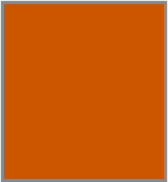
- Then we use convert_image_dtype() to convert our image data into float32. This is only done for the images, not the mask, since the mask was already decoded into float32. There are two common data types used in image processing: float32 and uint8. Float32 stands for a floating point number (decimal) that occupies 32 bits in computer memory. They are signed (meaning the number can be negative) and can range in value from 0 to 2³² = 4294967296, although by convention in image processing we normalize these values to be between 0 and 1, where 1 is the maximum of a color. Uint8 stands for an unsigned (positive) integer that goes between 0 and 255 and only occupies 8 bits in memory. For example, we can represent the color burnt orange as (Red: 204, Green: 85, Blue: 0) for uint8 or (Red: 0.8, Green: 0.33, Blue: 0) for float32. Float32 is usually the better choice, since it offers more precision and already comes normalized which helps improve training. However, uint8 saves memory, and this can be better depending on your memory limitations. Using float32 in convert_image_dtype automatically normalizes the values.
- In binary segmentation, we expect our masks to have shape (batch, hieght, width, channels), with channels = 1. In other words, we want one class (car) being represented by the number 1, and the other class (background) being represented by the number 0. There is no reason for the number of channels to be 3, as in for RGB images. Unfortunately, after decoding it comes with three channels, with the class number repeated three times. To fix this, we use tf.math.reduce_max(mask, axis=-1, keepdims=True) to take the maximum of the values in the three channels and get rid of the rest. So a channel value of (1,1,1) gets reduced to just (1) and a channel value of (0,0,0) gets reduced to (0).
- Finally we resize the images/masks to our desired dimensions (small). Note that the images I showed earlier of the car with the ground truth mask look blurry; this downscaling was done on purpose to reduce the computational load and allow training to occur relatively quickly. Using method=‘nearest’ as a default is a good idea; otherwise the function will always return a float32, which is bad if you want it to be in uint8.

The color burnt orange can be represented in float32 or uint8 format. Image by author.
Once we have our datasets organized, we can now view our images:
# View images and associated labels
for images, masks in batched_val_dataset.take(1):
car_number = 0
for image_slot in range(16):
ax = plt.subplot(4, 4, image_slot + 1)
if image_slot % 2 == 0:
plt.imshow((images[car_number]))
class_name = 'Image'
else:
plt.imshow(masks[car_number], cmap = 'gray')
plt.colorbar()
class_name = 'Mask'
car_number += 1
plt.title(class_name)
plt.axis("off")

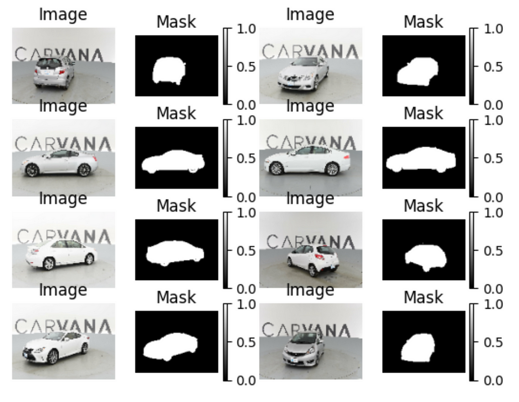
Images of our cars paired with the accompanying masks.
Here we are using the .take() method to view the first batch of data in our batched_val_dataset. Since we are doing binary segmentation, we want our mask to only contain two values: 0 and 1. Plotting the color bars on the mask confirms we have the right setup. Note that we added the argument cmap = ‘gray’ to the mask imshow() to let plt know we want these images presented in grayscale.
Building a Simple U-Net Model
In a letter dated February 5, 1675 to his rival Robert Hooke, Isaac Newton stated:
“If I have seen further, it is by standing on the shoulders of giants.”
In this same vein, we will stand on the shoulders of previous machine learning researchers who have discovered what sorts of architectures work best for the task of image segmentation. It is not a bad idea to experiment with architectures of your own; however, the researchers who have come before us have gone down many dead ends to discover the models that work. These architectures aren’t necessarily the end all be all, as research is still ongoing and a better architecture may yet be found.

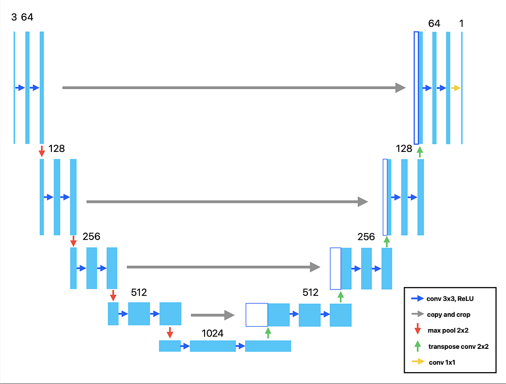
Visualization of the U-Net, described in [1]. Image by author.
One of the more well-known architectures is called the U-Net, so called because the downsampling and the upsampling portions of the network can be visualized as a U (see below). In a paper titled U-Net: Convolutional Networks for Biomedical Image Segmentation by Ronneberger, Fisher, and Brox [1], the authors describe how to create a fully convolutional network (FCN) that works effectively for image segmentation. Fully convolutional means there are no densely connected layers; all the layers are convolutional.
There are a few things to note:
- The network consists of a series of repeating blocks of two convolutional layers, with padding = ‘same’ and stride = 1 so that the outputs of the convolutions are not downsized within the block.
- Each block is followed by a max pooling layer, which cuts down the width and height of the feature map in half.
- The next block then doubles the number of filters. And the pattern continues. This pattern of cutting the feature space down while increasing the number of filters should be familiar if you have studied CNNs. This completes what the authors call the “contracting path.”
- The “bottleneck” layer is at the bottom of the ‘U’. This layer captures highly abstracted features (lines, curves, windows, doors, etc.) but at a significantly reduced spatial resolution.
- Next begins what they call the “expanding path.” In short, this reverses the contractions, with each block consisting again of two convolutional layers. Each block is followed by an upsampling layer, which in TensorFlow we call the Conv2DTranspose layer. This takes a smaller feature map and doubles the height and width.
- The next block then cuts the number of filters in half. Repeat the process until you wind up with the same height and width as the images you started with. Finally, finish with a 1x1 conv layer to reduce the number of channels to 1. We want to finish with one channel because this is binary segmentation, so we desire a single filter where the pixel values correspond to our two classes. We use a sigmoid activation to smush the pixel values between 0 and 1.
- There are also skip connections in the U-Net architecture, allowing the network to retain fine-grained spatial information even after downsampling and then upsampling. Normally there is a lot of information lost in this process. By passing the information from a contracting block and into the corresponding expanding block, we can preserve this spatial information. There is a nice symmetry to the architecture.
We will begin by doing a simple version of the U-Net. This will be a FCN, but with no residual connections and no max pooling layers.
data_augmentation = tf.keras.Sequential([
tfl.RandomFlip(mode="horizontal", seed=42),
tfl.RandomRotation(factor=0.01, seed=42),
tfl.RandomContrast(factor=0.2, seed=42)
])
def get_model(img_size):
inputs = Input(shape=img_size + (3,))
x = data_augmentation(inputs)
# Contracting path
x = tfl.Conv2D(64, 3, strides=2, activation="relu", padding="same", kernel_initializer='he_normal')(x)
x = tfl.Conv2D(64, 3, activation="relu", padding="same", kernel_initializer='he_normal')(x)
x = tfl.Conv2D(128, 3, strides=2, activation="relu", padding="same", kernel_initializer='he_normal')(x)
x = tfl.Conv2D(128, 3, activation="relu", padding="same", kernel_initializer='he_normal')(x)
x = tfl.Conv2D(256, 3, strides=2, padding="same", activation="relu", kernel_initializer='he_normal')(x)
x = tfl.Conv2D(256, 3, activation="relu", padding="same", kernel_initializer='he_normal')(x)
# Expanding path
x = tfl.Conv2DTranspose(256, 3, activation="relu", padding="same", kernel_initializer='he_normal')(x)
x = tfl.Conv2DTranspose(256, 3, activation="relu", padding="same", kernel_initializer='he_normal', strides=2)(x)
x = tfl.Conv2DTranspose(128, 3, activation="relu", padding="same", kernel_initializer='he_normal')(x)
x = tfl.Conv2DTranspose(128, 3, activation="relu", padding="same", kernel_initializer='he_normal', strides=2)(x)
x = tfl.Conv2DTranspose(64, 3, activation="relu", padding="same", kernel_initializer='he_normal')(x)
x = tfl.Conv2DTranspose(64, 3, activation="relu", padding="same", kernel_initializer='he_normal', strides=2)(x)
outputs = tfl.Conv2D(1, 3, activation="sigmoid", padding="same")(x)
model = keras.Model(inputs, outputs)
return model
custom_model = get_model(img_size=img_size)
Here we have the same basic structure as the U-Net, with a contracting path and an expansion path. One interesting thing to note is that rather than use a max pooling layer to cut the feature space in half, we use a convolutional layer with strides=2. According to Chollet [2], this cuts the feature space in half while preserving more spatial information than a max pooling layers. He states that whenever location information is important (as in image segmentation) it is a good idea to avoid destructive max pooling layers and stick to using strided convolutions instead (this is curious, because the famous U-Net architecture does use max pooling). Also observe that we are doing some data augmentation to help our model generalize to unseen examples.
Some important details: setting the kernel_intializer to ‘he_normal’ setting for ReLU activations makes a surprisingly large difference in terms of training stability. I initially underestimated the power of kernel initialization. Rather than initializing the weights randomly, he_normalization initializes the weights to have a mean of 0 and a standard deviation of the square root of (2 / # of input units to layer). In the case of CNNs the number of input units refers to the number of channels in the feature maps of the previous layer. This has been found to lead to faster convergence, mitigate vanishing gradients, and improve learning. See reference [3] for more details.
Metrics and Loss Function
There are several common metrics and loss functions one can use for binary segmentation. Here, we will use the dice coefficient as a metric and the corresponding dice loss for training, as this is what the competition requires.
Let’s first take a look at the mathematics behind the dice coefficient:

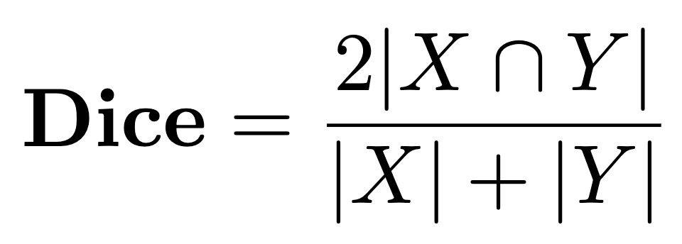
The dice coefficient, in the general form.
The dice coefficient is defined as the intersection between two sets (X and Y), divided by the sum of each set, multiplied by 2. The dice coefficient will lie between 0 (if the sets have no intersection) and 1 (if the sets overlap perfectly). Now we see why this makes a great metric for image segmentation.

An example of two masks overlayed over each other. Orange used for clarity. Image by author.
The above equation is a general definition of the dice coefficient; when when you apply it to vector quantities (as opposed to sets), we use the more specific definition:

The dice coefficient, in the vector form.
Here, we are iterating over each element (pixel) in each mask. x represents the ith pixel in the predicted mask and y represents the corresponding pixel in the ground truth mask. On top we are doing the element-wise product, and on bottom we are summing over all elements in each mask independently. N represents the total number of pixels (which should be the same for both predicted and target masks.) Remember that in our masks, the numbers will all be either 0s or 1s, so a pixel with a value of 1 in the ground truth mask and a corresponding pixel in the predicted mask with a value of 0 will not contribute to the dice score, as expected (1 x 0 = 0).
The dice loss will be simply defined as 1 — Dice Score. Since the dice score is between 0 and 1, the dice loss will also be between 0 and 1. In fact the sum of the dice score and the dice loss must equal 1. They are inversely related.
Let’s take a look at how this is implemented in code:
from tensorflow.keras import backend as K
def dice_coef(y_true, y_pred, smooth=10e-6):
y_true_f = K.flatten(y_true)
y_pred_f = K.flatten(y_pred)
intersection = K.sum(y_true_f * y_pred_f)
dice = (2. * intersection + smooth) / (K.sum(y_true_f) + K.sum(y_pred_f) + smooth)
return dice
def dice_loss(y_true, y_pred):
return 1 - dice_coef(y_true, y_pred)
Here we are flattening two 4-D masks (batch, height, width, channels=1) into 1-D vectors, and computing the dice scores for all images in the batch. Note that we adding a smoothing value to both the numerator and denominator to prevent having a 0/0 issue if the two masks do not overlap.
Finally, we begin training. We are doing early stopping to prevent overfitting and saving the best model.
custom_model.compile(optimizer=tf.keras.optimizers.Adam(learning_rate=0.0001,
epsilon=1e-06),
loss=[dice_loss],
metrics=[dice_coef])
callbacks_list = [
keras.callbacks.EarlyStopping(
monitor="val_loss",
patience=2,
),
keras.callbacks.ModelCheckpoint(
filepath="best-custom-model",
monitor="val_loss",
save_best_only=True,
)
]
history = custom_model.fit(batched_train_dataset, epochs=20,
callbacks=callbacks_list,
validation_data=batched_val_dataset)
We can determine the results of our training with the following code:
def display(display_list):
plt.figure(figsize=(15, 15))
title = ['Input Image', 'True Mask', 'Predicted Mask']
for i in range(len(display_list)):
plt.subplot(1, len(display_list), i+1)
plt.title(title)
plt.imshow(tf.keras.preprocessing.image.array_to_img(display_list))
plt.axis('off')
plt.show()
def create_mask(pred_mask):
mask = pred_mask[..., -1] >= 0.5
pred_mask[..., -1] = tf.where(mask, 1, 0)
# Return only first mask of batch
return pred_mask[0]
def show_predictions(model, dataset=None, num=1):
"""
Displays the first image of each of the num batches
"""
if dataset:
for image, mask in dataset.take(num):
pred_mask = model.predict(image)
display([image[0], mask[0], create_mask(pred_mask)])
else:
display([sample_image, sample_mask,
create_mask(model.predict(sample_image[tf.newaxis, ...]))])
custom_model = keras.models.load_model("/kaggle/working/best-custom-model", custom_objects={'dice_coef': dice_coef, 'dice_loss': dice_loss})
show_predictions(model = custom_model, dataset = batched_train_dataset, num = 6)
After 10 epochs, we arrive at a top validation dice score of 0.8788. Not terrible, but not great. On a P100 GPU this took me about 20 minutes. Here is a sample mask for our review:

Comparison of input image, true mask, and predicted mask. By the author.
Highlighting a few interesting points:
- Note that create_mask is the function that pushes pixel values to either 0 or 1. A pixel value of < 0.5 will will be cut to 0 and we will assign that pixel to the “background” category. A value ≥ 0.5 will be increased to 1 and we will call assign that pixel to the “car” category.
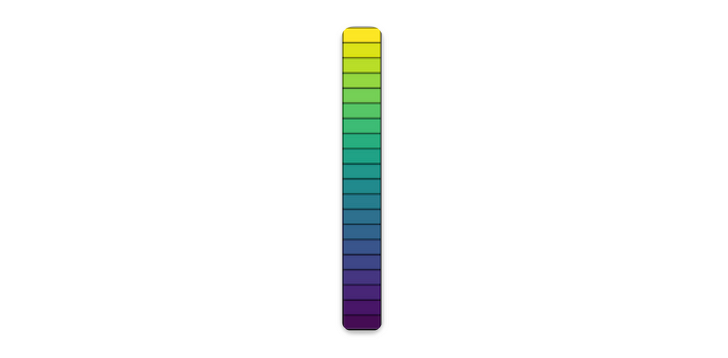
- Why did the masks come out yellow and purple, instead of black and white? We used: tf.keras.preprocessing.image.array_to_img() to converts the output of the mask from a tensor to a PIL Image. We then passed the image to plt.imshow(). From the documentation we see that that the default colormap for single channel images is “viridis” (3-channel RGB images get output as is.) The viridis colormap transforms low values to a deep purple and a high values to yellow. This colormap can apparently help people with colorblindness get an accurate view of the color in an image. We could’ve fixed this by adding cmap=“grayscale” as an argument, but this would’ve messed up our input image. See more here at this link.

The viridis colormap, from low values (purple) to high values (yellow). By the author.
Building the Complete U-Net
Now we turn to using the full U-Net architecture, with residual connections, max pooling layers, and including dropout layers for regularization. Note the contracting path, bottleneck layer, and expanding path. The dropout layers can be added in the contracting path, at the end of each block.
def conv_block(inputs=None, n_filters=64, dropout_prob=0, max_pooling=True):
conv = Conv2D(n_filters,
3,
activation='relu',
padding='same',
kernel_initializer='he_normal')(inputs)
conv = Conv2D(n_filters,
3,
activation='relu',
padding='same',
kernel_initializer='he_normal')(conv)
if dropout_prob > 0:
conv = Dropout(dropout_prob)(conv)
if max_pooling:
next_layer = MaxPooling2D(pool_size=(2, 2))(conv)
else:
next_layer = conv
skip_connection = conv
return next_layer, skip_connection
def upsampling_block(expansive_input, contractive_input, n_filters=64):
up = Conv2DTranspose(
n_filters,
3,
strides=(2, 2),
padding='same',
kernel_initializer='he_normal')(expansive_input)
# Merge the previous output and the contractive_input
merge = concatenate([up, contractive_input], axis=3)
conv = Conv2D(n_filters,
3,
activation='relu',
padding='same',
kernel_initializer='he_normal')(merge)
conv = Conv2D(n_filters,
3,
activation='relu',
padding='same',
kernel_initializer='he_normal')(conv)
return conv
def unet_model(input_size=(96, 128, 3), n_filters=64, n_classes=1):
inputs = Input(input_size)
inputs = data_augmentation(inputs)
# Contracting Path (encoding)
cblock1 = conv_block(inputs, n_filters)
cblock2 = conv_block(cblock1[0], n_filters*2)
cblock3 = conv_block(cblock2[0], n_filters*4)
cblock4 = conv_block(cblock3[0], n_filters*8, dropout_prob=0.3)
# Bottleneck Layer
cblock5 = conv_block(cblock4[0], n_filters*16, dropout_prob=0.3, max_pooling=False)
# Expanding Path (decoding)
ublock6 = upsampling_block(cblock5[0], cblock4[1], n_filters*8)
ublock7 = upsampling_block(ublock6, cblock3[1], n_filters*4)
ublock8 = upsampling_block(ublock7, cblock2[1], n_filters*2)
ublock9 = upsampling_block(ublock8, cblock1[1], n_filters)
conv9 = Conv2D(n_filters,
3,
activation='relu',
padding='same',
kernel_initializer='he_normal')(ublock9)
conv10 = Conv2D(n_classes, 1, padding='same', activation="sigmoid")(conv9)
model = tf.keras.Model(inputs=inputs, outputs=conv10)
return model
We then take compile the U-Net. I am using 64 filters for the first conv block. This is a hyperparameter that you would want to tune for optimal results.
unet = unet_model(input_size=(img_height, img_width, num_channels), n_filters=64, n_classes=1)
unet.compile(optimizer=tf.keras.optimizers.Adam(learning_rate=0.0001, epsilon=1e-06),
loss=[dice_loss],
metrics=[dice_coef])
callbacks_list = [
keras.callbacks.EarlyStopping(
monitor="val_loss",
patience=2,
),
keras.callbacks.ModelCheckpoint(
filepath="best-u_net-model",
monitor="val_loss",
save_best_only=True,
)
]
history = unet.fit(batched_train_dataset, epochs=20,
callbacks=callbacks_list,
validation_data=batched_val_dataset)
After 16 epochs, I get a validation dice score of 0.9416, much better then with the simple U-Net. This shouldn’t be too surprising; looking at the parameter count we have an order of magnitude increase from the simple U-Net to the complete U-Net. On a P100 GPU this took me about 32 minutes. We then take a peek at the predictions:
unet = keras.models.load_model("/kaggle/working/best-u_net-model", custom_objects={'dice_coef': dice_coef, 'dice_loss': dice_loss})
show_predictions(model = unet, dataset = batched_train_dataset, num = 6)

Predicted mask for the complete U-Net. Much better! By the author.
These predictions are much better. One thing to note from looking at multiple predictions is that the antenna sticking out of the cars is tough for the network. Given that the images are very pixelated, I can’t blame the network for missing this.
To improve performance, one would look at tweaking hyperparameters including:
- Number of downsampling and upsampling blocks
- Number of filters
- Image resolution
- Size of training set
- Loss function (perhaps combining dice loss with binary cross-entropy loss)
- Adjusting optimizer parameters. Training stability seems to be an issue for both models. From the documentation for the Adam optimizer: “The default value of 1e-7 for epsilon might not be a good default in general.” Increasing epsilon by an order of magnitude or more may help with training stability.
We can already see the road to an excellent score on the Carvana challenge. Too bad it’s already over!
Summary
This article was a deep dive on the topic of image segmentation, specifically binary segmentation. If you take anything away, remember the following:
- The goal of image segmentation is to find a mapping from input pixel values in an image to output numbers that your model can use to assign classes to each pixel.
- One of the first steps is to organize your images into TensorFlow Dataset objects and take a look at your images and corresponding masks.
- There is no need to re-invent the wheel when it comes to model architecture: we know from experience that a U-Net works well.
- The dice score is a common metric that is used for monitoring the success of your model’s predictions. We can also get our loss function from this.
Future work could go into converting the max pooling layers in the canonical U-Net architecture into strided convolutional layers.
Best of luck on your image segmentation problems!
References
[1] O. Ronneberger, P. Fischer, and T. Brox, U-Net: Convolutional Networks for Biomedical Image Segmentation (2015), MICCAI 2015 International Conference
[2] F. Chollet, Deep Learning with Python (2021), Manning Publications Co.
[3] K. He, X. Zhang, S. Ren, J. Sun, Delving Deep into Rectifiers: Surpassing Human-Level Performance on ImageNet Classification (2015), International Conference on Computer Vision (ICCV)
Image Segmentation: An In-Depth Guide was originally published in Towards Data Science on Medium, where people are continuing the conversation by highlighting and responding to this story.
