From data to decisions: maximizing rewards with policy improvement methods for optimal strategies

Introduction
Reinforcement learning is a domain in machine learning that introduces the concept of an agent who must learn optimal strategies in complex environments. The agent learns from its actions that result in rewards given the environment’s state. Reinforcement learning is a difficult topic and differs significantly from other areas of machine learning. That is why it should only be used when a given problem cannot be solved otherwise.
The incredible flexibility of reinforcement learning is that the same algorithms can be used to make the agent adapt to completely different, unknown, and complex conditions.
Reinforcement Learning, Part 1: Introduction and Main Concepts
About this article
In Part 1, we have introduced the main concepts of reinforcement learning: the framework, policies and value functions. The Bellman equation that recursively establishes the relationship of value functions is the backbone of modern algorithms. We will understand its power in this article by learning how it can be used to find optimal policies.
Let us imagine that we perfectly know the environment’s dynamics that contains |S| states. Action transition probablities are given by a policy π. Given that, we can solve the Bellman equation for the V-function for this environment that will, in fact, represent a system of linear equations with |S| variables (in case of the Q-function there will be |S| x |A| equations).
The solution to that system of equations corresponds to v-values for every state (or q-values for every pair (state, pair)).
Example
Let us have a look at a simple example of an environment with 5 states where T is a terminal state. Numbers in blue represent transition probabilities while number in red represent rewards received by the agent. We will also assume that the same action chosen by the agent in the state A (represented by the horizontal arrow with probability p = 0.6) leads to either C or D with different probabilities (p = 0.8 and p = 0.2).
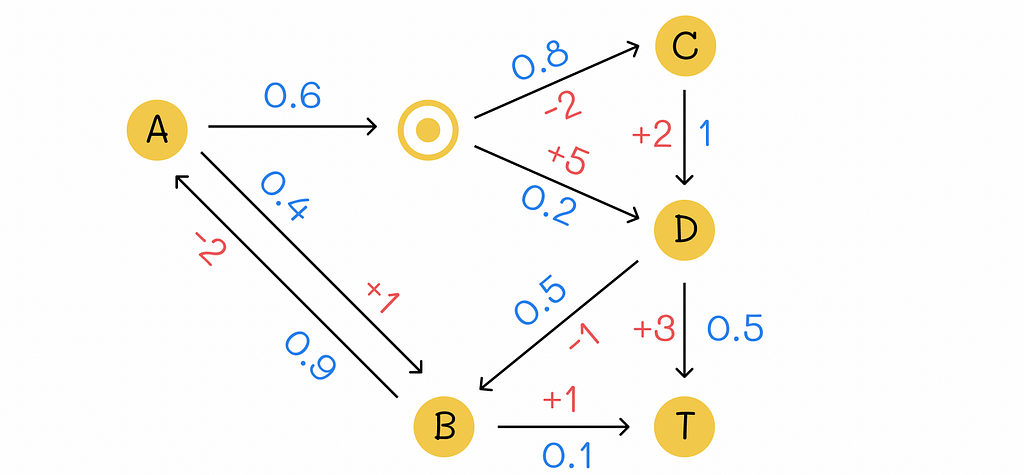
Transition diagram for the example. Numbers in blue denote transition probabilities between states and numbers in red define respective rewards.
Since the environment contains |S| = 5 states, to find all v-values, we will have to solve a system of equations consisting of 5 Bellman equations:
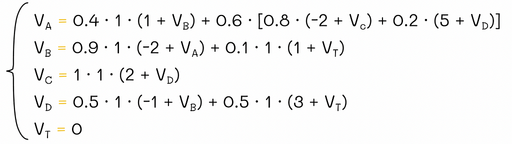
System of Bellman equations for the V-function.
Since T is a terminal state, its v-value is always 0, so technically we only have to solve 4 equations.
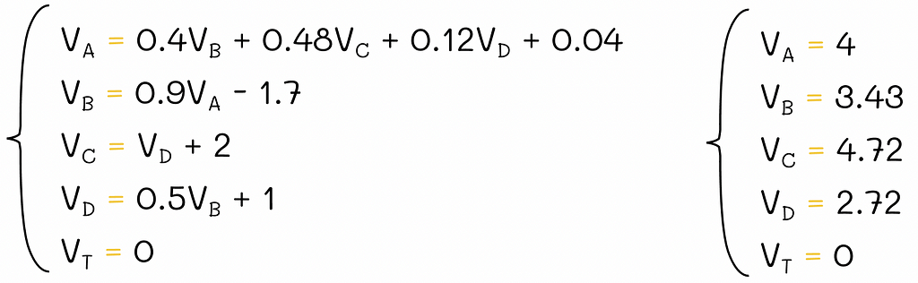
Solution of the system of equations.
Solving the analogous system for the Q-function would be harder because we would need to solve an equation for every pair (state, action).
Policy evaluation
Solving a linear system of equations in a straightforward manner, as it was shown in the example above, is a possible way to get real v-values. However, given the cubic algorithm complexity O(n³), where n = |S|, it is not optimal, especially when the number of states |S| is large. Instead, we can apply an iterative policy evaluation algorithm:
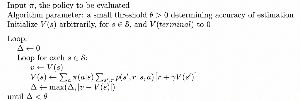
Policy evaluation pseudocode. Source: Reinforcement Learning. An Introduction. Second Edition | Richard S. Sutton and Andrew G. Barto
If the number of states |S| if finite, then it is possible to prove mathematically that iterative estimations obtained by the policy evaluation algorithm under a given policy π ultimately converge to real v-values!
To realize how amazing this algorithm is, let us highlight it once again:
The update equation in the policy evaluation algorithm can be implemented in two ways:
In practice, overwriting v-values is a preferable way to perform updates because the new information is used as soon as it becomes available for other updates, in comparison to the two array method. As a consequence, v-values tend to converge faster.
Description
To further understand how the policy evaluation algorithm works in practice, let us have a look at the example 4.1 from the Sutton’s and Barto’s book. We are given an environment in the form of the 4 x 4 grid where at every step the agent equiprobably (p = 0.25) makes a single step in one of the four directions (up, right, down, left).
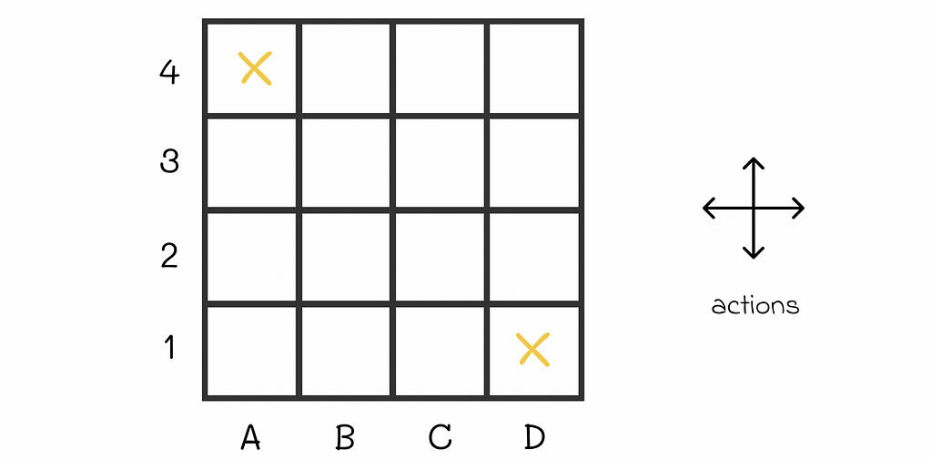
The agent starts at a random maze cell and can go in one of four directions receiving the reward R = -1 at every step. A4 and D1 are terminal states. Image adapted by the author. Source: Reinforcement Learning. An Introduction. Second Edition | Richard S. Sutton and Andrew G. Barto
If an agent is located at the edge of the maze and chooses to go into the direction of a wall around the maze, then its position stays the same. For example, if the agent is located at D3 and chooses to go to the right, then it will stay at D3 at the next state.
Every move to any cell results in R = -1 reward except for two terminal states located at A4 and D1 whose rewards are R = 0. The ultimate goal is to calculate V-function for the given equiprobable policy.
Algorithm
Let us initialize all V-values to 0. Then we will run several iterations of the policy evaluation algorithm:

The V-function on different policy evaluation iterations. Image adapted by the author. Source: Reinforcement Learning. An Introduction. Second Edition | Richard S. Sutton and Andrew G. Barto
At some point, there will be no changes between v-values on consecutive iterations. That means that the algorithm has converged to the real V-values. For the maze, the V-function under the equiprobable policy is shown at the right of the last diagram row.
Interpretation
Let us say an agent acting according to the random policy starts from the cell C2 whose expected reward is -18. By the V-function definition, -18 is the total cumulative reward the agent receives by the end of the episode. Since every move in the maze adds -1 to the reward, we can interpret the v-value of 18 as the expected number of steps the agent will have to make until it gets to the terminal state.
Policy improvement
At first sight, it might sound surprising but V- and Q- functions can be used to find optimal policies. To understand this, let us refer to the maze example where we have calculated the V-function for a starting random policy.
For instance, let us take the cell B3. Given our random policy, the agent can go in 4 directions with equal probabilities from that state. The possible expected rewards it can receive are -14, -20, -20 and -14. Let us suppose that we had an option to modify the policy for that state. To maximize the expected reward, would not it be logical to always go next to either A3 or B4 from B3, i.e. in the cell with the maximum expected reward in the neighbourhood (-14 in our case)?
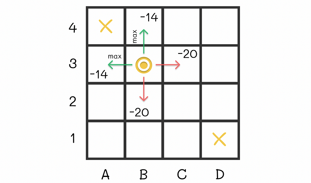
Optimal actions from the cell B3 lead to either A3 or B4 where the expected reward reaches its maximum.
This idea makes sense because being located at A3 or B4 gives the agent a possibility to finish the maze in just one step. As a result, we can include that transition rule for B3 to derive a new policy. Nevertheless, is it always optimal to make such transitions to maximize the expected reward?
To continue our example, let us perform the same procedure for all maze states:
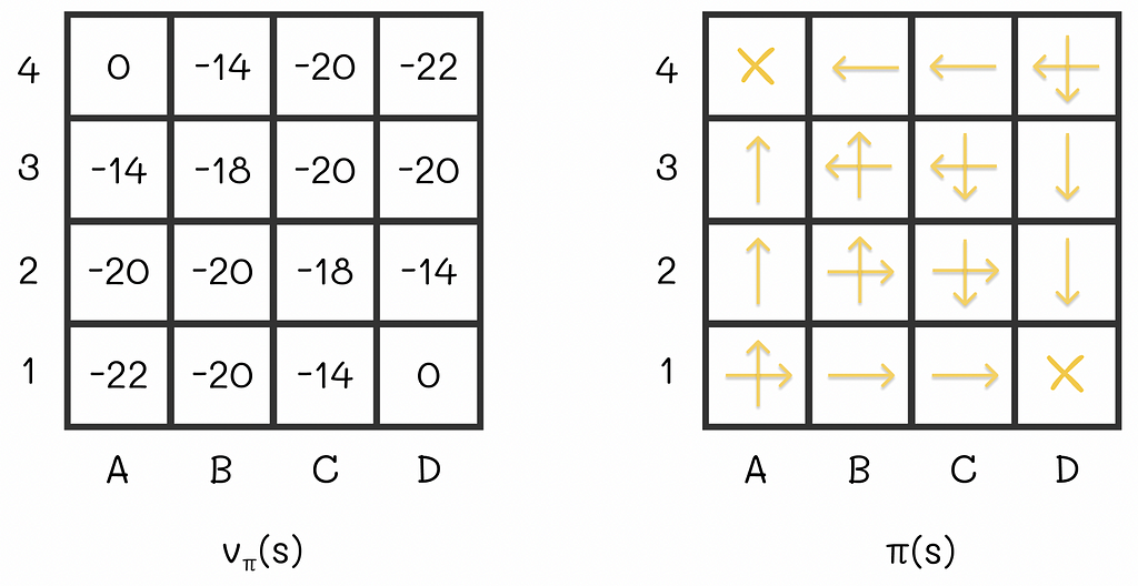
Converged V-function and its corresponding greedy policy from the example. Image adapted by the author. Source: Reinforcement Learning. An Introduction. Second Edition | Richard S. Sutton and Andrew G. Barto
As a consequence, we have derived a new policy that is better than the old one. By the way, our findings can be generalized for other problems as well by the policy improvement theorem which plays a crucial role in reinforcement learning.
Policy improvement theorem
Formulation
The formulation from the Sutton’s and Barto’s book concisely describes the theorem:

Source: Reinforcement Learning. An Introduction. Second Edition | Richard S. Sutton and Andrew G. Barto

Source: Reinforcement Learning. An Introduction. Second Edition | Richard S. Sutton and Andrew G. Barto
Logic
To understand the theorem’s formulation, let us assume that we have access to the V- and Q-functions of a given environment evaluated under a policy π. For that environment, we will create another policy π’. This policy will be absolutely the same as π with the only difference that for every state it will choose actions that result in either the same or greater rewards. Then the theorem guarantees that the V-function under policy π’ will be better than the one for the policy π.
Given any starting policy π, we can compute its V-function. This V-function can be used to improve the policy to π’. With this policy π’, we can calculate its V’-function. This procedure can be repeated multiple times to iteratively produce better policies and value functions.
In the limit, for a finite number of states, this algorithm, called policy iteration, converges to the optimal policy and the optimal value function.

The iterative alternation between policy evaluation (E) and policy improvement (I). Image adapted by the author. Source: Reinforcement Learning. An Introduction. Second Edition | Richard S. Sutton and Andrew G. Barto
If we applied the policy iteration algorithm to the maze example, then the optimal V-function and policy would look like this:
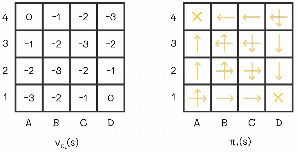
the optimal V-function and policy for the maze example. Image adapted by the author. Source: Reinforcement Learning. An Introduction. Second Edition | Richard S. Sutton and Andrew G. Barto
In these settings, with the obtained optimal V-function, we can easily estimate the number of steps required to get to the terminal state, according to the optimal strategy.
What is so interesting about this example is the fact that we would only need two policy iterations to obtain these values from scratch (we can notice that the optimal policy from the image is exactly the same as it was before when we had greedily updated it to the respective V-function). In some situations, the policy iteration algorithm requires only few iterations to converge.
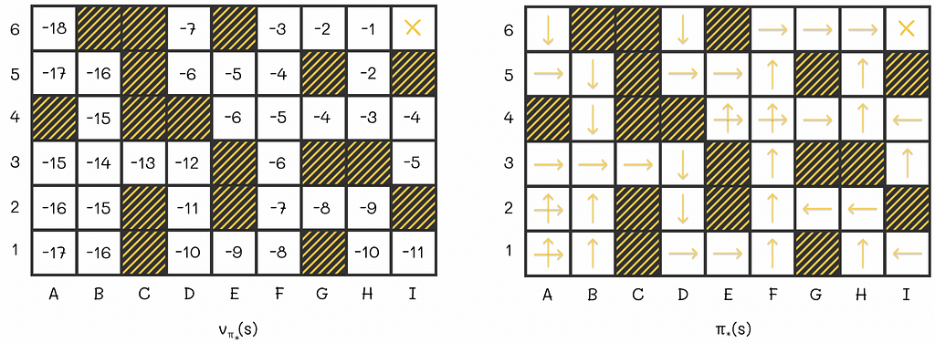
An example of the optimal V-function and policy for a more complex maze environment.
Value iteration
Though the original policy iteration algorithm can be used to find optimal policies, it can be slow, mainly because of multiple sweeps performed during policy evaluation steps. Moreover, the full convergence process to the exact V-function might require a lot sweeps.
In addition, sometimes it is not necessary to get exact v-values to yield a better policy. The previous example demonstrates it perfectly: instead of performing multiple sweeps, we could have done only k = 3 sweeps and then built a policy based on the obtained approximation of the V-function. This policy would have been exactly the same as the one we have computed after V-function convergence.
V-function and policy evaluations on the first three iterations. We can see that starting from the third iteration, the policy does not change. This example demonstrates that in some cases it is not necessary to run all iterations of policy iteration. Image adapted by the author. Source: Reinforcement Learning. An Introduction. Second Edition | Richard S. Sutton and Andrew G. Barto
In general, is it possible to stop the policy evaluation algorithm at some point? It turns out that yes! Furthermore, only a single sweep can be performed during every policy evaluation step and the result will still converge to the optimal policy. The described algorithm is called value iteration.
We are not going to study the proof of this algorithm. Nevertheless, we can notice that policy evaluation and policy improvement are two very similar processes to each other: both of them use the Bellman equation except for the fact that policy improvement takes the max operation to yield a better action.
By iteratively performing a single sweep of policy evaluation and a single sweep of policy improvement, we can converge faster to the optimum. In reality, we can stop the algorithm once the difference between successive V-functions becomes insignificant.
Asynchronous value iteration
In some situations, performing just a single sweep during every step of value iteration can be problematic, especially when the number of states |S| is large. To overcome this, asynchronous versions of the algorithm can be used: instead of systematically performing updates of all states during the whole sweep, only a subset of state values is updated in-place in whatever order. Moreover, some states can be updated multiple times before other states are updated.
However, at some point, all of the states will have to be updated, to make it possible for the algorithm to converge. According to the theory, all of the states must be updated in total an infinite number of times to achieve convergence but in practice this aspect is usually omitted since we are not always interested in getting 100% optimal policy.
There exist different implementations of asynchronous value iteration. In real problems, they make it possible to efficiently trade off between the algorithm’s speed and accuracy.
We have looked at the policy iteration algorithm. Its idea can be used to refer to a broader term in reinforcement learning called generalized policy iteration (GPI).
Sutton and Barto provide a simplified geometric figure that intuitively explains how GPI works. Let us imagine a 2D plane where every point represents a combination of a value function and a policy. Then we will draw two lines:
Geometric visualisation of policy improvement towards the optimality point. Image adapted by the author. Source: Reinforcement Learning. An Introduction. Second Edition | Richard S. Sutton and Andrew G. Barto
Every time when we calculate a greedy policy for the current V-function, we move closer to the policy line while moving away from the V-function line. That is logical because for the new computed policy, the previous V-function no longer applies. On the other hand, every time we perform policy evaluation, we move towards the projection of a point on the V-function line and thus we move further from the policy line: for the new estimated V-function, the current policy is no longer optimal. The whole process is repeated again.
As these two processes alternate between each other, both current V-function and policy gradually improve and at some moment in time they must reach a point of optimality that will represent an intersection between the V-function and policy lines.
Conclusion
In this article, we have gone through the main ideas behind policy evaluation and policy improvement. The beauty of these two algorithms is their ability to interact with each other to reach the optimal state. This approach only works in perfect environments where the agent’s probability transitions are given for all states and actions. Despite this constraint, many other reinforcement learning algorithms use the GPI method as a fundamental building block for finding optimal policies.
For environments with numerous states, several heuristics can be applied to accelerate the convergence speed one of which includes asynchronous updates during the policy evaluation step. Since the majority of reinforcement algorithms require a lot of computational resources, this technique becomes very useful and allows efficiently trading accuracy for gains in speed.
Resources
All images unless otherwise noted are by the author.

Reinforcement Learning, Part 2: Policy Evaluation and Improvement was originally published in Towards Data Science on Medium, where people are continuing the conversation by highlighting and responding to this story.
Introduction
Reinforcement learning is a domain in machine learning that introduces the concept of an agent who must learn optimal strategies in complex environments. The agent learns from its actions that result in rewards given the environment’s state. Reinforcement learning is a difficult topic and differs significantly from other areas of machine learning. That is why it should only be used when a given problem cannot be solved otherwise.
The incredible flexibility of reinforcement learning is that the same algorithms can be used to make the agent adapt to completely different, unknown, and complex conditions.
Note. To fully understand the ideas included in this article, it is highly recommended to be familiar with the main concepts of reinforcement learning introduced in the first part of this article series.
Reinforcement Learning, Part 1: Introduction and Main Concepts
About this article
In Part 1, we have introduced the main concepts of reinforcement learning: the framework, policies and value functions. The Bellman equation that recursively establishes the relationship of value functions is the backbone of modern algorithms. We will understand its power in this article by learning how it can be used to find optimal policies.
This article is based on Chapter 4 of the book “Reinforcement Learning” written by Richard S. Sutton and Andrew G. Barto. I highly appreciate the efforts of the authors who contributed to the publication of this book.
Solving Bellman equationLet us imagine that we perfectly know the environment’s dynamics that contains |S| states. Action transition probablities are given by a policy π. Given that, we can solve the Bellman equation for the V-function for this environment that will, in fact, represent a system of linear equations with |S| variables (in case of the Q-function there will be |S| x |A| equations).
The solution to that system of equations corresponds to v-values for every state (or q-values for every pair (state, pair)).
Example
Let us have a look at a simple example of an environment with 5 states where T is a terminal state. Numbers in blue represent transition probabilities while number in red represent rewards received by the agent. We will also assume that the same action chosen by the agent in the state A (represented by the horizontal arrow with probability p = 0.6) leads to either C or D with different probabilities (p = 0.8 and p = 0.2).
Transition diagram for the example. Numbers in blue denote transition probabilities between states and numbers in red define respective rewards.
Since the environment contains |S| = 5 states, to find all v-values, we will have to solve a system of equations consisting of 5 Bellman equations:
System of Bellman equations for the V-function.
Since T is a terminal state, its v-value is always 0, so technically we only have to solve 4 equations.
Solution of the system of equations.
Solving the analogous system for the Q-function would be harder because we would need to solve an equation for every pair (state, action).
Policy evaluation
Solving a linear system of equations in a straightforward manner, as it was shown in the example above, is a possible way to get real v-values. However, given the cubic algorithm complexity O(n³), where n = |S|, it is not optimal, especially when the number of states |S| is large. Instead, we can apply an iterative policy evaluation algorithm:
- Randomly initialise v-values for all environment states (except for terminal states whose v-values must be equal to 0).
- Iteratively update all non-terminal states by using the Bellman equation.
- Repeat step 2 until the difference between previous and current v-values is too small (≤ θ).
Policy evaluation pseudocode. Source: Reinforcement Learning. An Introduction. Second Edition | Richard S. Sutton and Andrew G. Barto
If the number of states |S| if finite, then it is possible to prove mathematically that iterative estimations obtained by the policy evaluation algorithm under a given policy π ultimately converge to real v-values!
A single update of the v-value of a state s ∈ S is called an expected update. The logic behind this name is that the update procedure considers rewards of all possible successive states of s, not just a single one.
A whole iteration of updates for all states is called a sweep.
Note. The analogous iterative algorithm can be applied to the calculation of Q-functions as well.
To realize how amazing this algorithm is, let us highlight it once again:
Policy evaluation allows iteratively finding the V-function under a given policy π.
Update variationsThe update equation in the policy evaluation algorithm can be implemented in two ways:
- By using two arrays: new values are computed sequentially from unchanged old values stored in two separate arrays.
- By using one array: computed values are overwritten immediately. As a result, later updates during the same iteration use the overwritten new values.
In practice, overwriting v-values is a preferable way to perform updates because the new information is used as soon as it becomes available for other updates, in comparison to the two array method. As a consequence, v-values tend to converge faster.
The algorithm does not impose rules on the order of variables that should be updated during every iteration, however the order can have a large influence on the convergence rate.
ExampleDescription
To further understand how the policy evaluation algorithm works in practice, let us have a look at the example 4.1 from the Sutton’s and Barto’s book. We are given an environment in the form of the 4 x 4 grid where at every step the agent equiprobably (p = 0.25) makes a single step in one of the four directions (up, right, down, left).
The agent starts at a random maze cell and can go in one of four directions receiving the reward R = -1 at every step. A4 and D1 are terminal states. Image adapted by the author. Source: Reinforcement Learning. An Introduction. Second Edition | Richard S. Sutton and Andrew G. Barto
If an agent is located at the edge of the maze and chooses to go into the direction of a wall around the maze, then its position stays the same. For example, if the agent is located at D3 and chooses to go to the right, then it will stay at D3 at the next state.
Every move to any cell results in R = -1 reward except for two terminal states located at A4 and D1 whose rewards are R = 0. The ultimate goal is to calculate V-function for the given equiprobable policy.
Algorithm
Let us initialize all V-values to 0. Then we will run several iterations of the policy evaluation algorithm:
The V-function on different policy evaluation iterations. Image adapted by the author. Source: Reinforcement Learning. An Introduction. Second Edition | Richard S. Sutton and Andrew G. Barto
At some point, there will be no changes between v-values on consecutive iterations. That means that the algorithm has converged to the real V-values. For the maze, the V-function under the equiprobable policy is shown at the right of the last diagram row.
Interpretation
Let us say an agent acting according to the random policy starts from the cell C2 whose expected reward is -18. By the V-function definition, -18 is the total cumulative reward the agent receives by the end of the episode. Since every move in the maze adds -1 to the reward, we can interpret the v-value of 18 as the expected number of steps the agent will have to make until it gets to the terminal state.
Policy improvement
At first sight, it might sound surprising but V- and Q- functions can be used to find optimal policies. To understand this, let us refer to the maze example where we have calculated the V-function for a starting random policy.
For instance, let us take the cell B3. Given our random policy, the agent can go in 4 directions with equal probabilities from that state. The possible expected rewards it can receive are -14, -20, -20 and -14. Let us suppose that we had an option to modify the policy for that state. To maximize the expected reward, would not it be logical to always go next to either A3 or B4 from B3, i.e. in the cell with the maximum expected reward in the neighbourhood (-14 in our case)?
Optimal actions from the cell B3 lead to either A3 or B4 where the expected reward reaches its maximum.
This idea makes sense because being located at A3 or B4 gives the agent a possibility to finish the maze in just one step. As a result, we can include that transition rule for B3 to derive a new policy. Nevertheless, is it always optimal to make such transitions to maximize the expected reward?
Indeed, transitioning greedily to the state with an action whose combination of expected reward is maximal among other possible next states, leads to a better policy.
To continue our example, let us perform the same procedure for all maze states:
Converged V-function and its corresponding greedy policy from the example. Image adapted by the author. Source: Reinforcement Learning. An Introduction. Second Edition | Richard S. Sutton and Andrew G. Barto
As a consequence, we have derived a new policy that is better than the old one. By the way, our findings can be generalized for other problems as well by the policy improvement theorem which plays a crucial role in reinforcement learning.
Policy improvement theorem
Formulation
The formulation from the Sutton’s and Barto’s book concisely describes the theorem:
Let π and π’ be any pair of deterministic policies such that, for all s ∈ S,
Source: Reinforcement Learning. An Introduction. Second Edition | Richard S. Sutton and Andrew G. Barto
Then the policy π’ must be as good as, or better than, π. That is, it must obtain greater or equal expected return from all states s ∈ S:
Source: Reinforcement Learning. An Introduction. Second Edition | Richard S. Sutton and Andrew G. Barto
Logic
To understand the theorem’s formulation, let us assume that we have access to the V- and Q-functions of a given environment evaluated under a policy π. For that environment, we will create another policy π’. This policy will be absolutely the same as π with the only difference that for every state it will choose actions that result in either the same or greater rewards. Then the theorem guarantees that the V-function under policy π’ will be better than the one for the policy π.
With the policy improvement theorem, we can always derive better policies by greedily choosing actions of the current policy that lead to maximum rewards for every state.
Policy iterationGiven any starting policy π, we can compute its V-function. This V-function can be used to improve the policy to π’. With this policy π’, we can calculate its V’-function. This procedure can be repeated multiple times to iteratively produce better policies and value functions.
In the limit, for a finite number of states, this algorithm, called policy iteration, converges to the optimal policy and the optimal value function.
The iterative alternation between policy evaluation (E) and policy improvement (I). Image adapted by the author. Source: Reinforcement Learning. An Introduction. Second Edition | Richard S. Sutton and Andrew G. Barto
If we applied the policy iteration algorithm to the maze example, then the optimal V-function and policy would look like this:
the optimal V-function and policy for the maze example. Image adapted by the author. Source: Reinforcement Learning. An Introduction. Second Edition | Richard S. Sutton and Andrew G. Barto
In these settings, with the obtained optimal V-function, we can easily estimate the number of steps required to get to the terminal state, according to the optimal strategy.
What is so interesting about this example is the fact that we would only need two policy iterations to obtain these values from scratch (we can notice that the optimal policy from the image is exactly the same as it was before when we had greedily updated it to the respective V-function). In some situations, the policy iteration algorithm requires only few iterations to converge.
An example of the optimal V-function and policy for a more complex maze environment.
Value iteration
Though the original policy iteration algorithm can be used to find optimal policies, it can be slow, mainly because of multiple sweeps performed during policy evaluation steps. Moreover, the full convergence process to the exact V-function might require a lot sweeps.
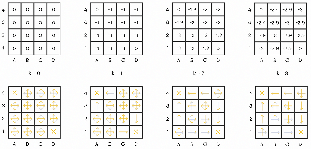
In addition, sometimes it is not necessary to get exact v-values to yield a better policy. The previous example demonstrates it perfectly: instead of performing multiple sweeps, we could have done only k = 3 sweeps and then built a policy based on the obtained approximation of the V-function. This policy would have been exactly the same as the one we have computed after V-function convergence.
V-function and policy evaluations on the first three iterations. We can see that starting from the third iteration, the policy does not change. This example demonstrates that in some cases it is not necessary to run all iterations of policy iteration. Image adapted by the author. Source: Reinforcement Learning. An Introduction. Second Edition | Richard S. Sutton and Andrew G. Barto
In general, is it possible to stop the policy evaluation algorithm at some point? It turns out that yes! Furthermore, only a single sweep can be performed during every policy evaluation step and the result will still converge to the optimal policy. The described algorithm is called value iteration.
We are not going to study the proof of this algorithm. Nevertheless, we can notice that policy evaluation and policy improvement are two very similar processes to each other: both of them use the Bellman equation except for the fact that policy improvement takes the max operation to yield a better action.
By iteratively performing a single sweep of policy evaluation and a single sweep of policy improvement, we can converge faster to the optimum. In reality, we can stop the algorithm once the difference between successive V-functions becomes insignificant.
Asynchronous value iteration
In some situations, performing just a single sweep during every step of value iteration can be problematic, especially when the number of states |S| is large. To overcome this, asynchronous versions of the algorithm can be used: instead of systematically performing updates of all states during the whole sweep, only a subset of state values is updated in-place in whatever order. Moreover, some states can be updated multiple times before other states are updated.
However, at some point, all of the states will have to be updated, to make it possible for the algorithm to converge. According to the theory, all of the states must be updated in total an infinite number of times to achieve convergence but in practice this aspect is usually omitted since we are not always interested in getting 100% optimal policy.
There exist different implementations of asynchronous value iteration. In real problems, they make it possible to efficiently trade off between the algorithm’s speed and accuracy.
One of the the simplest asynchronous versions is to update only a single state during the policy evaluation.
Generalized policy iterationWe have looked at the policy iteration algorithm. Its idea can be used to refer to a broader term in reinforcement learning called generalized policy iteration (GPI).
The GPI consists of finding the optimal policy through independent alternation between policy evaluation and policy improvement processes.
Almost all of the reinforcement learning algorithms can be referred to as GPI.
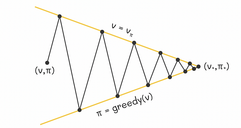
Sutton and Barto provide a simplified geometric figure that intuitively explains how GPI works. Let us imagine a 2D plane where every point represents a combination of a value function and a policy. Then we will draw two lines:
- The first line will contain points corresponding to different V-functions of an environment.
- The second line will represent a set of greedy policies in relation to respective V-functions.
Geometric visualisation of policy improvement towards the optimality point. Image adapted by the author. Source: Reinforcement Learning. An Introduction. Second Edition | Richard S. Sutton and Andrew G. Barto
Every time when we calculate a greedy policy for the current V-function, we move closer to the policy line while moving away from the V-function line. That is logical because for the new computed policy, the previous V-function no longer applies. On the other hand, every time we perform policy evaluation, we move towards the projection of a point on the V-function line and thus we move further from the policy line: for the new estimated V-function, the current policy is no longer optimal. The whole process is repeated again.
As these two processes alternate between each other, both current V-function and policy gradually improve and at some moment in time they must reach a point of optimality that will represent an intersection between the V-function and policy lines.
Conclusion
In this article, we have gone through the main ideas behind policy evaluation and policy improvement. The beauty of these two algorithms is their ability to interact with each other to reach the optimal state. This approach only works in perfect environments where the agent’s probability transitions are given for all states and actions. Despite this constraint, many other reinforcement learning algorithms use the GPI method as a fundamental building block for finding optimal policies.
For environments with numerous states, several heuristics can be applied to accelerate the convergence speed one of which includes asynchronous updates during the policy evaluation step. Since the majority of reinforcement algorithms require a lot of computational resources, this technique becomes very useful and allows efficiently trading accuracy for gains in speed.
Resources
All images unless otherwise noted are by the author.
Reinforcement Learning, Part 2: Policy Evaluation and Improvement was originally published in Towards Data Science on Medium, where people are continuing the conversation by highlighting and responding to this story.