Decoding the Math behind Reinforcement Learning, introducing the RL Framework, and building one RL simulation from scratch in Python.

Image generated by DALL-E
Reinforcement learning (RL) stands as a pivotal element in the landscape of artificial intelligence, known for its unique method of teaching machines to make decisions through their own experiences within an environment. In this article, we’re going to take a deep dive into what makes RL tick. We’ll break down its core concepts, highlight the broad range of its applications, decode the math, and guide you through building it from scratch.
Index
· Introduction to Reinforcement Learning
∘ What is Reinforcement Learning?
∘ How does it work?
· The RL Framework
∘ States
∘ Actions
∘ Rewards
· The Concept of Episodes and Policy
∘ Episodes
∘ Policy
· Mathematical Formulation of the RL Problem
∘ Objective Function
∘ Return (Cumulative Reward)
∘ Discounting
· Building an RL Environment
· Next Steps
∘ Current Shortcomings
∘ Expanding Horizons: The Road Ahead
· Conclusion
Introduction to Reinforcement Learning
What is Reinforcement Learning?

Image generated by DALL-E
Reinforcement learning, or RL, is an area of artificial intelligence that’s all about teaching machines to make smart choices. Think of it as similar to training a dog. You give treats to encourage the behaviors you like, and over time, the dog — or in this case, a computer program — figures out which actions get the best results. But instead of yummy treats, we use numerical rewards, and the machine’s goal is to score as high as it can.
Now, your dog might not be a champ at board games, but RL can outsmart world champions. Take the time Google’s DeepMind introduced AlphaGo. This RL-powered software went head-to-head with Lee Sedol, a top player in the game Go, and won back in 2016. AlphaGo got better by playing loads of games against both human and computer opponents, learning and improving with each game.
But RL isn’t just for beating game champions. It’s also making waves in robotics, helping robots learn tasks that are tough to code directly, like grabbing and moving objects. And it’s behind the personalized recommendations you get on platforms like Netflix and Spotify, tweaking its suggestions to match what you like.
How does it work?
At the core of reinforcement learning (RL) is this dynamic between an agent (that’s you or the algorithm) and its environment. Picture this: you’re playing a video game. You’re the agent, the game’s world is the environment, and your mission is to rack up as many points as possible. Every moment in the game is a chance to make a move, and depending on what you do, the game throws back a new scenario and maybe some rewards (like points for snagging a coin or knocking out an enemy).
This give-and-take keeps going, with the agent (whether it’s you or the algorithm) figuring out which moves bring in the most rewards as time goes on. It’s all about trial and error, where the machine slowly but surely uncovers the best game plan, or policy, to hit its targets.
RL is a bit different from other ways of learning machines, like supervised learning, where a model learns from a set of data that already has the right answers, or unsupervised learning, which is all about spotting patterns in data without clear-cut instructions. With RL, there’s no cheat sheet. The agent learns purely through its adventures — making choices, seeing what happens, and learning from it.
This article is just the beginning of our “Reinforcement Learning 101” series. We’re going to break down the essentials of reinforcement learning, from the basic ideas to the intricate algorithms that power some of the most sophisticated AI out there. And here’s the fun part: you’ll get to try your hand at coding these concepts in Python, starting with our very first article. So, whether you’re a student, a developer, or just someone fascinated by AI, this series will give you the tools and knowledge to dive into the thrilling realm of reinforcement learning.
Let’s get started!
The RL Framework
Let’s dive deeper into the heart of reinforcement learning, where everything revolves around the interaction between an agent and its environment. This relationship is all about a cycle of actions, states, and rewards, helping the agent learn the best way to act over time. Here’s a simple breakdown of these crucial elements:
States
The state is a snapshot of the environment at any given moment. It’s the backdrop against which decisions are made. In a video game, a state might show where all the players and objects are on the screen. States can range from something straightforward like a robot’s location on a grid, to something complex like the many factors that describe the stock market at any time.
Mathematically, we often write a state as s ∈ S, where S is the set of all possible states. States can be either discrete (like the spot of a character on a grid) or continuous (like the speed and position of a car).
To make this more clear, imagine a simple 5x5 grid. Here, states are where the agent is on the grid, marked by coordinates (x,y), with x being the row and y the column. In a 5x5 grid, there are 25 possible spots, from the top-left corner (0,0) to the bottom-right (4,4), covering everything in between.
Let’s say the agent’s mission is to navigate from a starting point to a goal, dodging obstacles along the way. Picture this grid: the start is a yellow block at the top-left, the goal is a light grey block at the bottom-right, and there are pink blocks as obstacles.
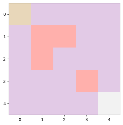
Grid Environment — Image by Author
In a bit of code to set up this scenario, we’d define the grid’s size (5x5), the start point (0,0), the goal (4,4), and any obstacles. The agent’s current state starts at the beginning point, and we sprinkle in some obstacles for an extra challenge.
class GridWorld:
def __init__(self, width: int = 5, height: int = 5, start: tuple = (0, 0), goal: tuple = (4, 4), obstacles: list = None):
self.width = width
self.height = height
self.start = np.array(start)
self.goal = np.array(goal)
self.obstacles = [np.array(obstacle) for obstacle in obstacles] if obstacles else []
self.state = self.start
Here’s a peek at what that setup might look like in code. We set the grid to be 5x5, with the starting point at (0,0) and the goal at (4,4). We keep track of the agent’s current spot with self.state, starting at the start point. And we add obstacles to mix things up.
If this snippet of code seems a bit much right now, no worries! We’ll dive into a detailed example later on, making everything crystal clear.
Actions
Actions are what an agent can do to change its current state. If we stick with the video game example, actions might include moving left or right, jumping, or doing something specific like shooting. The collection of all actions an agent can take at any point is known as the action space. This space can be discrete, meaning there’s a set number of actions, or continuous, where actions can vary within a range.
In math terms, we express an action as a ∈ A(s), where A represents the action space, and A(s) is the set of all possible actions in state s. Actions can be either discrete or continuous, just like states.
Going back to our simpler grid example, let’s define our possible moves:
action_effects = {'up': (-1, 0), 'down': (1, 0), 'left': (0, -1), 'right': (0, 1)}
Each action is represented by a tuple showing the change in position. So, to move down from the starting point (0,0) to (1,0), you’d adjust one row down. To move right, you go from (1,0) to (1,1) by changing one column. To transition from one state to the next, we simply add the action’s effect to the current position.
However, our grid world has boundaries and obstacles to consider, so we’ve got to make sure our moves don’t lead us out of bounds or into trouble. Here’s how we handle that:
# Check for boundaries and obstacles
if 0 <= next_state[0] < self.height and 0 <= next_state[1] < self.width and next_state not in self.obstacles:
self.state = next_state
This piece of code checks if the next move keeps us within the grid and avoids obstacles. If it does, the agent can proceed to that next spot.
So, actions are all about making moves and navigating the environment, considering what’s possible and what’s off-limits due to the layout and rules of our grid world.
Rewards
Rewards are like instant feedback that the agent gets from the environment after it makes a move. Think of them as points that show whether an action was beneficial or not. The agent’s main aim is to collect as many points as possible over time, which means it has to think about both the short-term gains and the long-term impacts of its actions. Just like we mentioned earlier with the dog training analogy when a dog does something good, we give it a treat; if not, there might be a mild telling-off. This idea is pretty much a staple in reinforcement learning.
Mathematically, we describe a reward that comes from making a move a in state s and moving to a new state s′ as R(s, a, s′). Rewards can be either positive (like a treat) or negative (more like a gentle scold), and they’re crucial for helping the agent learn the best actions to take.
In our grid world scenario, we want to give the agent a big thumbs up if it reaches its goal. And because we value efficiency, we’ll deduct points for every move it makes that doesn’t succeed. In code, we’d set up a reward system somewhat like this:
reward = 100 if (self.state == self.goal).all() else -1
This means the agent gets a whopping 100 points for landing on the goal but loses a point for every step that doesn’t get it there. It’s a simple way to encourage our agent to find the quickest route to its target.
The Concept of Episodes and Policy
Understanding episodes and policy is key to getting how agents learn and decide what to do in reinforcement learning (RL) environments. Let’s dive into these concepts:
Episodes
Think of an episode in reinforcement learning as a complete run of activity, starting from an initial point and ending when a specific goal is reached or a stopping condition is met. During an episode, the agent goes through a series of steps: it checks out the current situation (state), makes a move (action) based on its strategy (policy), and then gets feedback (reward) and the new situation (next state) from the environment. Episodes neatly package the agent’s experiences in scenarios where tasks have a clear start and finish.
In a video game, an episode might be tackling a single level, kicking off at the start of the level and wrapping up when the player either wins or runs out of lives.
In financial trading, an episode could be framed as a single trading day, starting when the market opens and ending at the close.
Episodes are useful because they let us measure how well different strategies (policies) work over a set period and help in learn from a full experience. This setup gives the agent chances to restart, apply what it’s learned, and experiment with new tactics under similar conditions.
Mathematically, you can visualize an episode as a series of moments:

Series of Moments — Image by Author
where:
This sequence helps in tracking the flow of actions, states, and rewards throughout an episode, providing a framework for learning and improving strategies.
Policy
In the world of reinforcement learning (RL), a policy is essentially the game plan an agent follows to decide its moves in different situations. It’s like a guidebook that maps out which actions to take when faced with various scenarios. Policies can come in two flavors: deterministic and stochastic.
Deterministic Policy
A deterministic policy is straightforward: for any specific situation, it tells the agent exactly what to do. If you find yourself in a state s, the policy has a predefined action a ready to go. This kind of policy always picks the same action for a given state, making it predictable. You can think of a deterministic policy as a direct function that links states to their corresponding actions:

Deterministic Policy Formula — Image by Author
where a is the action chosen when the agent is in state s.
Stochastic Policy
On the flip side, a stochastic policy adds a bit of unpredictability to the mix. Instead of a single action, it gives a set of probabilities for choosing among available actions in a given state. This randomness is crucial for exploring the environment, especially when the agent is still figuring out which actions work best. A stochastic policy is often expressed as a probability distribution over actions given a state s, symbolized as π(a ∣ s), indicating the likelihood of choosing action a when in state s:

Stochastic Policy Formula — Image by Author
where P denotes the probability.
The endgame of reinforcement learning is to uncover the optimal policy, one that maximizes the total expected rewards over time. Finding this balance between exploring new actions and exploiting known lucrative ones is key. The idea of an “optimal policy” ties closely to the value function concept, which gauges the anticipated rewards (or returns) from each state or action-state pairing, based on the policy in play. This journey of exploration and exploitation helps the agent learn the best paths to take, aiming for the highest cumulative reward.
Mathematical Formulation of the RL Problem
The way reinforcement learning (RL) problems are set up mathematically is key to understanding how agents learn to make smart decisions that maximize their rewards over time. This setup involves a few main ideas: the objective function, return (or cumulative reward), discounting, and the overall goal of optimization. Let’s dig into these concepts:
Objective Function
At the core of RL is the objective function, which is the target that the agent is trying to hit by interacting with the environment. Simply put, the agent wants to collect as many rewards as it can. We measure this goal using the expected return, which is the total of all rewards the agent thinks it can get, starting from a certain point and following a specific game plan or policy.
Return (Cumulative Reward)
“Return” is the term used for the total rewards that an agent picks up, whether that’s in one go (a single episode) or over a longer period. You can think of it as the agent’s score, where every move it makes either earns or loses points based on how well it turns out. If we’re not thinking about discounting for a moment, the return is just the sum of all rewards from each step t until the episode ends:

Return Formula — Image by Author
Here, Rt represents the reward obtained at time t, and T marks the episode’s conclusion.
Discounting
In RL, not every reward is seen as equally valuable. There’s a preference for rewards received sooner rather than later, and this is where discounting comes into play. Discounting reduces the value of future rewards with a discount factor γ, which is a number between 0 and 1. The discounted return formula looks like this:

Discounting Formula — Image by Author
This approach keeps the agent’s score from blowing up to infinity, especially when we’re looking at endless scenarios. It also encourages the agent to prioritize actions that deliver rewards more quickly, balancing the pursuit of immediate versus future gains.
Building an RL Environment
Now, let’s take the grid example we talked about earlier, and write a code to implement an agent navigating through the environment and reaching its goal. Let’s construct a straightforward grid world environment, outline a navigation policy for our agent, and kick off a simulation to see everything in action.
Let’s first show all the code and then let’s break it down.
import numpy as np
import matplotlib.pyplot as plt
import logging
logging.basicConfig(level=logging.INFO)
class GridWorld:
"""
GridWorld environment for navigation.
Args:
- width: Width of the grid
- height: Height of the grid
- start: Start position of the agent
- goal: Goal position of the agent
- obstacles: List of obstacles in the grid
Methods:
- reset: Reset the environment to the start state
- is_valid_state: Check if the given state is valid
- step: Take a step in the environment
"""
def __init__(self, width: int = 5, height: int = 5, start: tuple = (0, 0), goal: tuple = (4, 4), obstacles: list = None):
self.width = width
self.height = height
self.start = np.array(start)
self.goal = np.array(goal)
self.obstacles = [np.array(obstacle) for obstacle in obstacles] if obstacles else []
self.state = self.start
self.actions = {'up': np.array([-1, 0]), 'down': np.array([1, 0]), 'left': np.array([0, -1]), 'right': np.array([0, 1])}
def reset(self):
"""
Reset the environment to the start state
Returns:
- Start state of the environment
"""
self.state = self.start
return self.state
def is_valid_state(self, state):
"""
Check if the given state is valid
Args:
- state: State to be checked
Returns:
- True if the state is valid, False otherwise
"""
return 0 <= state[0] < self.height and 0 <= state[1] < self.width and all((state != obstacle).any() for obstacle in self.obstacles)
def step(self, action: str):
"""
Take a step in the environment
Args:
- action: Action to be taken
Returns:
- Next state, reward, done
"""
next_state = self.state + self.actions[action]
if self.is_valid_state(next_state):
self.state = next_state
reward = 100 if (self.state == self.goal).all() else -1
done = (self.state == self.goal).all()
return self.state, reward, done
def navigation_policy(state: np.array, goal: np.array, obstacles: list):
"""
Policy for navigating the agent in the grid world environment
Args:
- state: Current state of the agent
- goal: Goal state of the agent
- obstacles: List of obstacles in the environment
Returns:
- Action to be taken by the agent
"""
actions = ['up', 'down', 'left', 'right']
valid_actions = {}
for action in actions:
next_state = state + env.actions[action]
if env.is_valid_state(next_state):
valid_actions[action] = np.sum(np.abs(next_state - goal))
return min(valid_actions, key=valid_actions.get) if valid_actions else None
def run_simulation_with_policy(env: GridWorld, policy):
"""
Run the simulation with the given policy
Args:
- env: GridWorld environment
- policy: Policy to be used for navigation
"""
state = env.reset()
done = False
logging.info(f"Start State: {state}, Goal: {env.goal}, Obstacles: {env.obstacles}")
while not done:
# Visualization
grid = np.zeros((env.height, env.width))
grid[tuple(state)] = 1 # current state
grid[tuple(env.goal)] = 2 # goal
for obstacle in env.obstacles:
grid[tuple(obstacle)] = -1 # obstacles
plt.imshow(grid, cmap='Pastel1')
plt.show()
action = policy(state, env.goal, env.obstacles)
if action is None:
logging.info("No valid actions available, agent is stuck.")
break
next_state, reward, done = env.step(action)
logging.info(f"State: {state} -> Action: {action} -> Next State: {next_state}, Reward: {reward}")
state = next_state
if done:
logging.info("Goal reached!")
# Define obstacles in the environment
obstacles = [(1, 1), (1, 2), (2, 1), (3, 3)]
# Create the environment with obstacles
env = GridWorld(obstacles=obstacles)
# Run the simulation
run_simulation_with_policy(env, navigation_policy)
Link to full code:
Reinforcement-Learning/Tutorial 1 - Building your first RL Agent/demo.ipynb at main · cristianleoo/Reinforcement-Learning
GridWorld Class
class GridWorld:
def __init__(self, width: int = 5, height: int = 5, start: tuple = (0, 0), goal: tuple = (4, 4), obstacles: list = None):
self.width = width
self.height = height
self.start = np.array(start)
self.goal = np.array(goal)
self.obstacles = [np.array(obstacle) for obstacle in obstacles] if obstacles else []
self.state = self.start
self.actions = {'up': np.array([-1, 0]), 'down': np.array([1, 0]), 'left': np.array([0, -1]), 'right': np.array([0, 1])}
This class initializes a grid environment with a specified width and height, a start position for the agent, a goal position to reach, and a list of obstacles. Note that obstacles are a list of tuples, where each tuple represents the position of each obstacle.
Here, self.actions defines possible movements (up, down, left, right) as vectors that will modify the agent's position.
def reset(self):
self.state = self.start
return self.state
reset() method sets the agent's state back to the start position. This is useful when we want to train the agent several times, after each completion of the reach of a certain status, the agent will start back from the beginning.
def is_valid_state(self, state):
return 0 <= state[0] < self.height and 0 <= state[1] < self.width and all((state != obstacle).any() for obstacle in self.obstacles)
is_valid_state(state) checks if a given state is within the grid boundaries and not an obstacle.
def step(self, action: str):
next_state = self.state + self.actions[action]
if self.is_valid_state(next_state):
self.state = next_state
reward = 100 if (self.state == self.goal).all() else -1
done = (self.state == self.goal).all()
return self.state, reward, done
step(action: str) moves the agent according to the action if it's valid, updates the state, calculates the reward, and checks if the goal is reached.
Navigation Policy Function
def navigation_policy(state: np.array, goal: np.array, obstacles: list):
actions = ['up', 'down', 'left', 'right']
valid_actions = {}
for action in actions:
next_state = state + env.actions[action]
if env.is_valid_state(next_state):
valid_actions[action] = np.sum(np.abs(next_state - goal))
return min(valid_actions, key=valid_actions.get) if valid_actions else None
Defines a simple policy to decide the next action based on minimizing the distance to the goal while considering valid actions only. Indeed, for every valid action we calculate the distance between the new state and the goal, then we select the action that minimizes the distance. Keep in mind, that the function to calculate the distance is crucial for a performant RL agent. In this case, we are using a Manhattan distance calculation, but this may not be the best choice for different and more complex scenarios.
Simulation Function
def run_simulation_with_policy(env: GridWorld, policy):
state = env.reset()
done = False
logging.info(f"Start State: {state}, Goal: {env.goal}, Obstacles: {env.obstacles}")
while not done:
# Visualization
grid = np.zeros((env.height, env.width))
grid[tuple(state)] = 1 # current state
grid[tuple(env.goal)] = 2 # goal
for obstacle in env.obstacles:
grid[tuple(obstacle)] = -1 # obstacles
plt.imshow(grid, cmap='Pastel1')
plt.show()
action = policy(state, env.goal, env.obstacles)
if action is None:
logging.info("No valid actions available, agent is stuck.")
break
next_state, reward, done = env.step(action)
logging.info(f"State: {state} -> Action: {action} -> Next State: {next_state}, Reward: {reward}")
state = next_state
if done:
logging.info("Goal reached!")
run_simulation_with_policy(env: GridWorld, policy) resets the environment and iteratively applies the navigation policy to move the agent towards the goal. It visualizes the grid and the agent's progress at each step.
The simulation runs until the goal is reached or no valid actions are available (the agent is stuck).
Running the Simulation
# Define obstacles in the environment
obstacles = [(1, 1), (1, 2), (2, 1), (3, 3)]
# Create the environment with obstacles
env = GridWorld(obstacles=obstacles)
# Run the simulation
run_simulation_with_policy(env, navigation_policy)
The simulation is run using run_simulation_with_policy, applying the defined navigation policy to guide the agent.

Agent moving towards a goal — GIF by Author
By developing this RL environment and simulation, you get a firsthand look at the basics of agent navigation and decision-making, foundational concepts in the field of reinforcement learning.
Next Steps
As we delve deeper into the world of reinforcement learning (RL), it’s important to take stock of where we currently stand. Here’s a rundown of what our current approach lacks and our plans for bridging these gaps:
Current Shortcomings
Static Environment
Our simulations run in a fixed grid world, with unchanging obstacles and goals. This setup doesn’t challenge the agent with new or evolving obstacles, limiting its need to adapt or strategize beyond the basics.
Basic Navigation Policy
The policy we’ve implemented is quite basic, focusing solely on obstacle avoidance and goal achievement. It lacks the depth required for more complex decision-making or learning from past interactions with the environment.
No Learning Mechanism
As it stands, our agent doesn’t learn from its experiences. It reacts to immediate rewards without improving its approach based on past actions, missing out on the essence of RL: learning and improving over time.
Absence of MDP Framework
Our current model does not explicitly utilize the Markov Decision Process (MDP) framework. MDPs are crucial for understanding the dynamics of state transitions, actions, and rewards, and are foundational for advanced learning algorithms like Q-learning.
Expanding Horizons: The Road Ahead
Recognizing these limitations is the first step toward enhancing our RL exploration. Here’s what we plan to tackle in the next article:
Dynamic Environment
We’ll upgrade our grid world to introduce elements that change over time, such as moving obstacles or changing rewards. This will compel the agent to continuously adapt its strategies, offering a richer, more complex learning experience.
Implementing Q-learning
To give our agent the ability to learn and evolve, we’ll introduce Q-learning. This algorithm is a game-changer, enabling the agent to accumulate knowledge and refine its strategies based on the outcomes of past actions.
Exploring MDPs
Diving into the Markov Decision Process will provide a solid theoretical foundation for our simulations. Understanding MDPs is key to grasping decision-making in uncertain environments, evaluating and improving policies, and how algorithms like Q-learning fit into this framework.
Complex Algorithms and Strategies
With the groundwork laid by Q-learning and MDPs, we’ll explore more sophisticated algorithms and strategies. This advancement will not only elevate our agent’s intelligence but also its proficiency in navigating the intricacies of a dynamic and challenging grid world.
By addressing these areas, we aim to unlock new levels of complexity and learning in our reinforcement learning journey. The next steps promise to transform our simple agent into one capable of making informed decisions, adapting to changing environments, and continuously learning from its experiences.
Conclusion
Wrapping up our initial dive into the core concepts of reinforcement learning (RL) within the confines of a simple grid world, it’s clear we’ve only scratched the surface of what’s possible. This first article has set the stage, showcasing both the promise and the current constraints of our approach. The simplicity of our static setup and the basic nature of our navigation tactics have spotlighted key areas ready for advancement.
You made it to the end. Congrats! I hope you enjoyed this article. If so consider leaving a clap and following me, as I will regularly post similar articles. As with every beginning of a new series, this article may not be perfect, and with your input, it can highly improve. So, let me know what you think about it, what you would like to see more, and what less.

Reinforcement Learning 101: Building a RL Agent was originally published in Towards Data Science on Medium, where people are continuing the conversation by highlighting and responding to this story.
Image generated by DALL-E
Reinforcement learning (RL) stands as a pivotal element in the landscape of artificial intelligence, known for its unique method of teaching machines to make decisions through their own experiences within an environment. In this article, we’re going to take a deep dive into what makes RL tick. We’ll break down its core concepts, highlight the broad range of its applications, decode the math, and guide you through building it from scratch.
Index
· Introduction to Reinforcement Learning
∘ What is Reinforcement Learning?
∘ How does it work?
· The RL Framework
∘ States
∘ Actions
∘ Rewards
· The Concept of Episodes and Policy
∘ Episodes
∘ Policy
· Mathematical Formulation of the RL Problem
∘ Objective Function
∘ Return (Cumulative Reward)
∘ Discounting
· Building an RL Environment
· Next Steps
∘ Current Shortcomings
∘ Expanding Horizons: The Road Ahead
· Conclusion
Introduction to Reinforcement Learning
What is Reinforcement Learning?
Image generated by DALL-E
Reinforcement learning, or RL, is an area of artificial intelligence that’s all about teaching machines to make smart choices. Think of it as similar to training a dog. You give treats to encourage the behaviors you like, and over time, the dog — or in this case, a computer program — figures out which actions get the best results. But instead of yummy treats, we use numerical rewards, and the machine’s goal is to score as high as it can.
Now, your dog might not be a champ at board games, but RL can outsmart world champions. Take the time Google’s DeepMind introduced AlphaGo. This RL-powered software went head-to-head with Lee Sedol, a top player in the game Go, and won back in 2016. AlphaGo got better by playing loads of games against both human and computer opponents, learning and improving with each game.
But RL isn’t just for beating game champions. It’s also making waves in robotics, helping robots learn tasks that are tough to code directly, like grabbing and moving objects. And it’s behind the personalized recommendations you get on platforms like Netflix and Spotify, tweaking its suggestions to match what you like.
How does it work?
At the core of reinforcement learning (RL) is this dynamic between an agent (that’s you or the algorithm) and its environment. Picture this: you’re playing a video game. You’re the agent, the game’s world is the environment, and your mission is to rack up as many points as possible. Every moment in the game is a chance to make a move, and depending on what you do, the game throws back a new scenario and maybe some rewards (like points for snagging a coin or knocking out an enemy).
This give-and-take keeps going, with the agent (whether it’s you or the algorithm) figuring out which moves bring in the most rewards as time goes on. It’s all about trial and error, where the machine slowly but surely uncovers the best game plan, or policy, to hit its targets.
RL is a bit different from other ways of learning machines, like supervised learning, where a model learns from a set of data that already has the right answers, or unsupervised learning, which is all about spotting patterns in data without clear-cut instructions. With RL, there’s no cheat sheet. The agent learns purely through its adventures — making choices, seeing what happens, and learning from it.
This article is just the beginning of our “Reinforcement Learning 101” series. We’re going to break down the essentials of reinforcement learning, from the basic ideas to the intricate algorithms that power some of the most sophisticated AI out there. And here’s the fun part: you’ll get to try your hand at coding these concepts in Python, starting with our very first article. So, whether you’re a student, a developer, or just someone fascinated by AI, this series will give you the tools and knowledge to dive into the thrilling realm of reinforcement learning.
Let’s get started!
The RL Framework
Let’s dive deeper into the heart of reinforcement learning, where everything revolves around the interaction between an agent and its environment. This relationship is all about a cycle of actions, states, and rewards, helping the agent learn the best way to act over time. Here’s a simple breakdown of these crucial elements:
States
A state represents the current situation or configuration of the environment.
The state is a snapshot of the environment at any given moment. It’s the backdrop against which decisions are made. In a video game, a state might show where all the players and objects are on the screen. States can range from something straightforward like a robot’s location on a grid, to something complex like the many factors that describe the stock market at any time.
Mathematically, we often write a state as s ∈ S, where S is the set of all possible states. States can be either discrete (like the spot of a character on a grid) or continuous (like the speed and position of a car).
To make this more clear, imagine a simple 5x5 grid. Here, states are where the agent is on the grid, marked by coordinates (x,y), with x being the row and y the column. In a 5x5 grid, there are 25 possible spots, from the top-left corner (0,0) to the bottom-right (4,4), covering everything in between.
Let’s say the agent’s mission is to navigate from a starting point to a goal, dodging obstacles along the way. Picture this grid: the start is a yellow block at the top-left, the goal is a light grey block at the bottom-right, and there are pink blocks as obstacles.
Grid Environment — Image by Author
In a bit of code to set up this scenario, we’d define the grid’s size (5x5), the start point (0,0), the goal (4,4), and any obstacles. The agent’s current state starts at the beginning point, and we sprinkle in some obstacles for an extra challenge.
class GridWorld:
def __init__(self, width: int = 5, height: int = 5, start: tuple = (0, 0), goal: tuple = (4, 4), obstacles: list = None):
self.width = width
self.height = height
self.start = np.array(start)
self.goal = np.array(goal)
self.obstacles = [np.array(obstacle) for obstacle in obstacles] if obstacles else []
self.state = self.start
Here’s a peek at what that setup might look like in code. We set the grid to be 5x5, with the starting point at (0,0) and the goal at (4,4). We keep track of the agent’s current spot with self.state, starting at the start point. And we add obstacles to mix things up.
If this snippet of code seems a bit much right now, no worries! We’ll dive into a detailed example later on, making everything crystal clear.
Actions
Actions are the choices available to the agent that can change the state.
Actions are what an agent can do to change its current state. If we stick with the video game example, actions might include moving left or right, jumping, or doing something specific like shooting. The collection of all actions an agent can take at any point is known as the action space. This space can be discrete, meaning there’s a set number of actions, or continuous, where actions can vary within a range.
In math terms, we express an action as a ∈ A(s), where A represents the action space, and A(s) is the set of all possible actions in state s. Actions can be either discrete or continuous, just like states.
Going back to our simpler grid example, let’s define our possible moves:
action_effects = {'up': (-1, 0), 'down': (1, 0), 'left': (0, -1), 'right': (0, 1)}
Each action is represented by a tuple showing the change in position. So, to move down from the starting point (0,0) to (1,0), you’d adjust one row down. To move right, you go from (1,0) to (1,1) by changing one column. To transition from one state to the next, we simply add the action’s effect to the current position.
However, our grid world has boundaries and obstacles to consider, so we’ve got to make sure our moves don’t lead us out of bounds or into trouble. Here’s how we handle that:
# Check for boundaries and obstacles
if 0 <= next_state[0] < self.height and 0 <= next_state[1] < self.width and next_state not in self.obstacles:
self.state = next_state
This piece of code checks if the next move keeps us within the grid and avoids obstacles. If it does, the agent can proceed to that next spot.
So, actions are all about making moves and navigating the environment, considering what’s possible and what’s off-limits due to the layout and rules of our grid world.
Rewards
Rewards are immediate feedback received from the environment following an action.
Rewards are like instant feedback that the agent gets from the environment after it makes a move. Think of them as points that show whether an action was beneficial or not. The agent’s main aim is to collect as many points as possible over time, which means it has to think about both the short-term gains and the long-term impacts of its actions. Just like we mentioned earlier with the dog training analogy when a dog does something good, we give it a treat; if not, there might be a mild telling-off. This idea is pretty much a staple in reinforcement learning.
Mathematically, we describe a reward that comes from making a move a in state s and moving to a new state s′ as R(s, a, s′). Rewards can be either positive (like a treat) or negative (more like a gentle scold), and they’re crucial for helping the agent learn the best actions to take.
In our grid world scenario, we want to give the agent a big thumbs up if it reaches its goal. And because we value efficiency, we’ll deduct points for every move it makes that doesn’t succeed. In code, we’d set up a reward system somewhat like this:
reward = 100 if (self.state == self.goal).all() else -1
This means the agent gets a whopping 100 points for landing on the goal but loses a point for every step that doesn’t get it there. It’s a simple way to encourage our agent to find the quickest route to its target.
The Concept of Episodes and Policy
Understanding episodes and policy is key to getting how agents learn and decide what to do in reinforcement learning (RL) environments. Let’s dive into these concepts:
Episodes
An episode in reinforcement learning is a sequence of steps that starts in an initial state and ends when a terminal state is reached.
Think of an episode in reinforcement learning as a complete run of activity, starting from an initial point and ending when a specific goal is reached or a stopping condition is met. During an episode, the agent goes through a series of steps: it checks out the current situation (state), makes a move (action) based on its strategy (policy), and then gets feedback (reward) and the new situation (next state) from the environment. Episodes neatly package the agent’s experiences in scenarios where tasks have a clear start and finish.
In a video game, an episode might be tackling a single level, kicking off at the start of the level and wrapping up when the player either wins or runs out of lives.
In financial trading, an episode could be framed as a single trading day, starting when the market opens and ending at the close.
Episodes are useful because they let us measure how well different strategies (policies) work over a set period and help in learn from a full experience. This setup gives the agent chances to restart, apply what it’s learned, and experiment with new tactics under similar conditions.
Mathematically, you can visualize an episode as a series of moments:
Series of Moments — Image by Author
where:
- st is the state at the time t
- at is the action taken at the time t
- rt+1 is the reward received after the action at
- T marks the end of the episode
This sequence helps in tracking the flow of actions, states, and rewards throughout an episode, providing a framework for learning and improving strategies.
Policy
A policy is the strategy that an RL agent employs to decide which actions to take in various states.
In the world of reinforcement learning (RL), a policy is essentially the game plan an agent follows to decide its moves in different situations. It’s like a guidebook that maps out which actions to take when faced with various scenarios. Policies can come in two flavors: deterministic and stochastic.
Deterministic Policy
A deterministic policy is straightforward: for any specific situation, it tells the agent exactly what to do. If you find yourself in a state s, the policy has a predefined action a ready to go. This kind of policy always picks the same action for a given state, making it predictable. You can think of a deterministic policy as a direct function that links states to their corresponding actions:
Deterministic Policy Formula — Image by Author
where a is the action chosen when the agent is in state s.
Stochastic Policy
On the flip side, a stochastic policy adds a bit of unpredictability to the mix. Instead of a single action, it gives a set of probabilities for choosing among available actions in a given state. This randomness is crucial for exploring the environment, especially when the agent is still figuring out which actions work best. A stochastic policy is often expressed as a probability distribution over actions given a state s, symbolized as π(a ∣ s), indicating the likelihood of choosing action a when in state s:
Stochastic Policy Formula — Image by Author
where P denotes the probability.
The endgame of reinforcement learning is to uncover the optimal policy, one that maximizes the total expected rewards over time. Finding this balance between exploring new actions and exploiting known lucrative ones is key. The idea of an “optimal policy” ties closely to the value function concept, which gauges the anticipated rewards (or returns) from each state or action-state pairing, based on the policy in play. This journey of exploration and exploitation helps the agent learn the best paths to take, aiming for the highest cumulative reward.
Mathematical Formulation of the RL Problem
The way reinforcement learning (RL) problems are set up mathematically is key to understanding how agents learn to make smart decisions that maximize their rewards over time. This setup involves a few main ideas: the objective function, return (or cumulative reward), discounting, and the overall goal of optimization. Let’s dig into these concepts:
Objective Function
At the core of RL is the objective function, which is the target that the agent is trying to hit by interacting with the environment. Simply put, the agent wants to collect as many rewards as it can. We measure this goal using the expected return, which is the total of all rewards the agent thinks it can get, starting from a certain point and following a specific game plan or policy.
Return (Cumulative Reward)
“Return” is the term used for the total rewards that an agent picks up, whether that’s in one go (a single episode) or over a longer period. You can think of it as the agent’s score, where every move it makes either earns or loses points based on how well it turns out. If we’re not thinking about discounting for a moment, the return is just the sum of all rewards from each step t until the episode ends:
Return Formula — Image by Author
Here, Rt represents the reward obtained at time t, and T marks the episode’s conclusion.
Discounting
In RL, not every reward is seen as equally valuable. There’s a preference for rewards received sooner rather than later, and this is where discounting comes into play. Discounting reduces the value of future rewards with a discount factor γ, which is a number between 0 and 1. The discounted return formula looks like this:
Discounting Formula — Image by Author
This approach keeps the agent’s score from blowing up to infinity, especially when we’re looking at endless scenarios. It also encourages the agent to prioritize actions that deliver rewards more quickly, balancing the pursuit of immediate versus future gains.
Building an RL Environment
Now, let’s take the grid example we talked about earlier, and write a code to implement an agent navigating through the environment and reaching its goal. Let’s construct a straightforward grid world environment, outline a navigation policy for our agent, and kick off a simulation to see everything in action.
Let’s first show all the code and then let’s break it down.
import numpy as np
import matplotlib.pyplot as plt
import logging
logging.basicConfig(level=logging.INFO)
class GridWorld:
"""
GridWorld environment for navigation.
Args:
- width: Width of the grid
- height: Height of the grid
- start: Start position of the agent
- goal: Goal position of the agent
- obstacles: List of obstacles in the grid
Methods:
- reset: Reset the environment to the start state
- is_valid_state: Check if the given state is valid
- step: Take a step in the environment
"""
def __init__(self, width: int = 5, height: int = 5, start: tuple = (0, 0), goal: tuple = (4, 4), obstacles: list = None):
self.width = width
self.height = height
self.start = np.array(start)
self.goal = np.array(goal)
self.obstacles = [np.array(obstacle) for obstacle in obstacles] if obstacles else []
self.state = self.start
self.actions = {'up': np.array([-1, 0]), 'down': np.array([1, 0]), 'left': np.array([0, -1]), 'right': np.array([0, 1])}
def reset(self):
"""
Reset the environment to the start state
Returns:
- Start state of the environment
"""
self.state = self.start
return self.state
def is_valid_state(self, state):
"""
Check if the given state is valid
Args:
- state: State to be checked
Returns:
- True if the state is valid, False otherwise
"""
return 0 <= state[0] < self.height and 0 <= state[1] < self.width and all((state != obstacle).any() for obstacle in self.obstacles)
def step(self, action: str):
"""
Take a step in the environment
Args:
- action: Action to be taken
Returns:
- Next state, reward, done
"""
next_state = self.state + self.actions[action]
if self.is_valid_state(next_state):
self.state = next_state
reward = 100 if (self.state == self.goal).all() else -1
done = (self.state == self.goal).all()
return self.state, reward, done
def navigation_policy(state: np.array, goal: np.array, obstacles: list):
"""
Policy for navigating the agent in the grid world environment
Args:
- state: Current state of the agent
- goal: Goal state of the agent
- obstacles: List of obstacles in the environment
Returns:
- Action to be taken by the agent
"""
actions = ['up', 'down', 'left', 'right']
valid_actions = {}
for action in actions:
next_state = state + env.actions[action]
if env.is_valid_state(next_state):
valid_actions[action] = np.sum(np.abs(next_state - goal))
return min(valid_actions, key=valid_actions.get) if valid_actions else None
def run_simulation_with_policy(env: GridWorld, policy):
"""
Run the simulation with the given policy
Args:
- env: GridWorld environment
- policy: Policy to be used for navigation
"""
state = env.reset()
done = False
logging.info(f"Start State: {state}, Goal: {env.goal}, Obstacles: {env.obstacles}")
while not done:
# Visualization
grid = np.zeros((env.height, env.width))
grid[tuple(state)] = 1 # current state
grid[tuple(env.goal)] = 2 # goal
for obstacle in env.obstacles:
grid[tuple(obstacle)] = -1 # obstacles
plt.imshow(grid, cmap='Pastel1')
plt.show()
action = policy(state, env.goal, env.obstacles)
if action is None:
logging.info("No valid actions available, agent is stuck.")
break
next_state, reward, done = env.step(action)
logging.info(f"State: {state} -> Action: {action} -> Next State: {next_state}, Reward: {reward}")
state = next_state
if done:
logging.info("Goal reached!")
# Define obstacles in the environment
obstacles = [(1, 1), (1, 2), (2, 1), (3, 3)]
# Create the environment with obstacles
env = GridWorld(obstacles=obstacles)
# Run the simulation
run_simulation_with_policy(env, navigation_policy)
Link to full code:
Reinforcement-Learning/Tutorial 1 - Building your first RL Agent/demo.ipynb at main · cristianleoo/Reinforcement-Learning
GridWorld Class
class GridWorld:
def __init__(self, width: int = 5, height: int = 5, start: tuple = (0, 0), goal: tuple = (4, 4), obstacles: list = None):
self.width = width
self.height = height
self.start = np.array(start)
self.goal = np.array(goal)
self.obstacles = [np.array(obstacle) for obstacle in obstacles] if obstacles else []
self.state = self.start
self.actions = {'up': np.array([-1, 0]), 'down': np.array([1, 0]), 'left': np.array([0, -1]), 'right': np.array([0, 1])}
This class initializes a grid environment with a specified width and height, a start position for the agent, a goal position to reach, and a list of obstacles. Note that obstacles are a list of tuples, where each tuple represents the position of each obstacle.
Here, self.actions defines possible movements (up, down, left, right) as vectors that will modify the agent's position.
def reset(self):
self.state = self.start
return self.state
reset() method sets the agent's state back to the start position. This is useful when we want to train the agent several times, after each completion of the reach of a certain status, the agent will start back from the beginning.
def is_valid_state(self, state):
return 0 <= state[0] < self.height and 0 <= state[1] < self.width and all((state != obstacle).any() for obstacle in self.obstacles)
is_valid_state(state) checks if a given state is within the grid boundaries and not an obstacle.
def step(self, action: str):
next_state = self.state + self.actions[action]
if self.is_valid_state(next_state):
self.state = next_state
reward = 100 if (self.state == self.goal).all() else -1
done = (self.state == self.goal).all()
return self.state, reward, done
step(action: str) moves the agent according to the action if it's valid, updates the state, calculates the reward, and checks if the goal is reached.
Navigation Policy Function
def navigation_policy(state: np.array, goal: np.array, obstacles: list):
actions = ['up', 'down', 'left', 'right']
valid_actions = {}
for action in actions:
next_state = state + env.actions[action]
if env.is_valid_state(next_state):
valid_actions[action] = np.sum(np.abs(next_state - goal))
return min(valid_actions, key=valid_actions.get) if valid_actions else None
Defines a simple policy to decide the next action based on minimizing the distance to the goal while considering valid actions only. Indeed, for every valid action we calculate the distance between the new state and the goal, then we select the action that minimizes the distance. Keep in mind, that the function to calculate the distance is crucial for a performant RL agent. In this case, we are using a Manhattan distance calculation, but this may not be the best choice for different and more complex scenarios.
Simulation Function
def run_simulation_with_policy(env: GridWorld, policy):
state = env.reset()
done = False
logging.info(f"Start State: {state}, Goal: {env.goal}, Obstacles: {env.obstacles}")
while not done:
# Visualization
grid = np.zeros((env.height, env.width))
grid[tuple(state)] = 1 # current state
grid[tuple(env.goal)] = 2 # goal
for obstacle in env.obstacles:
grid[tuple(obstacle)] = -1 # obstacles
plt.imshow(grid, cmap='Pastel1')
plt.show()
action = policy(state, env.goal, env.obstacles)
if action is None:
logging.info("No valid actions available, agent is stuck.")
break
next_state, reward, done = env.step(action)
logging.info(f"State: {state} -> Action: {action} -> Next State: {next_state}, Reward: {reward}")
state = next_state
if done:
logging.info("Goal reached!")
run_simulation_with_policy(env: GridWorld, policy) resets the environment and iteratively applies the navigation policy to move the agent towards the goal. It visualizes the grid and the agent's progress at each step.
The simulation runs until the goal is reached or no valid actions are available (the agent is stuck).
Running the Simulation
# Define obstacles in the environment
obstacles = [(1, 1), (1, 2), (2, 1), (3, 3)]
# Create the environment with obstacles
env = GridWorld(obstacles=obstacles)
# Run the simulation
run_simulation_with_policy(env, navigation_policy)
The simulation is run using run_simulation_with_policy, applying the defined navigation policy to guide the agent.
Agent moving towards a goal — GIF by Author
By developing this RL environment and simulation, you get a firsthand look at the basics of agent navigation and decision-making, foundational concepts in the field of reinforcement learning.
Next Steps
As we delve deeper into the world of reinforcement learning (RL), it’s important to take stock of where we currently stand. Here’s a rundown of what our current approach lacks and our plans for bridging these gaps:
Current Shortcomings
Static Environment
Our simulations run in a fixed grid world, with unchanging obstacles and goals. This setup doesn’t challenge the agent with new or evolving obstacles, limiting its need to adapt or strategize beyond the basics.
Basic Navigation Policy
The policy we’ve implemented is quite basic, focusing solely on obstacle avoidance and goal achievement. It lacks the depth required for more complex decision-making or learning from past interactions with the environment.
No Learning Mechanism
As it stands, our agent doesn’t learn from its experiences. It reacts to immediate rewards without improving its approach based on past actions, missing out on the essence of RL: learning and improving over time.
Absence of MDP Framework
Our current model does not explicitly utilize the Markov Decision Process (MDP) framework. MDPs are crucial for understanding the dynamics of state transitions, actions, and rewards, and are foundational for advanced learning algorithms like Q-learning.
Expanding Horizons: The Road Ahead
Recognizing these limitations is the first step toward enhancing our RL exploration. Here’s what we plan to tackle in the next article:
Dynamic Environment
We’ll upgrade our grid world to introduce elements that change over time, such as moving obstacles or changing rewards. This will compel the agent to continuously adapt its strategies, offering a richer, more complex learning experience.
Implementing Q-learning
To give our agent the ability to learn and evolve, we’ll introduce Q-learning. This algorithm is a game-changer, enabling the agent to accumulate knowledge and refine its strategies based on the outcomes of past actions.
Exploring MDPs
Diving into the Markov Decision Process will provide a solid theoretical foundation for our simulations. Understanding MDPs is key to grasping decision-making in uncertain environments, evaluating and improving policies, and how algorithms like Q-learning fit into this framework.
Complex Algorithms and Strategies
With the groundwork laid by Q-learning and MDPs, we’ll explore more sophisticated algorithms and strategies. This advancement will not only elevate our agent’s intelligence but also its proficiency in navigating the intricacies of a dynamic and challenging grid world.
By addressing these areas, we aim to unlock new levels of complexity and learning in our reinforcement learning journey. The next steps promise to transform our simple agent into one capable of making informed decisions, adapting to changing environments, and continuously learning from its experiences.
Conclusion
Wrapping up our initial dive into the core concepts of reinforcement learning (RL) within the confines of a simple grid world, it’s clear we’ve only scratched the surface of what’s possible. This first article has set the stage, showcasing both the promise and the current constraints of our approach. The simplicity of our static setup and the basic nature of our navigation tactics have spotlighted key areas ready for advancement.
You made it to the end. Congrats! I hope you enjoyed this article. If so consider leaving a clap and following me, as I will regularly post similar articles. As with every beginning of a new series, this article may not be perfect, and with your input, it can highly improve. So, let me know what you think about it, what you would like to see more, and what less.
Reinforcement Learning 101: Building a RL Agent was originally published in Towards Data Science on Medium, where people are continuing the conversation by highlighting and responding to this story.